Statistical Methods#
Examples in this module use nx.les_miserables_graph().
All functions return scored full graphs; apply
threshold_filter() or
boolean_filter() as the second step.
Complexity classes are provided in each function docstring.
For a worked case study of scoring, choosing alpha and a correction,
and reporting, start with From a hairball to a backbone, end to end.
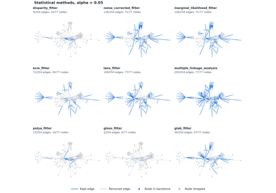
The tutorial Statistical null models side by side compares the null models on one
network, with figures.
Statistical backbone extraction methods.
These methods evaluate edge significance using hypothesis testing against
a null model. Each method computes a p-value (or score) for every edge,
which can then be filtered using functions in nx_backbone.filters.
Methods#
- disparity_filter
Serrano et al. (2009) – uniform distribution null model.
- noise_corrected_filter
Coscia & Neffke (2017) – Bayesian noise-corrected lift score.
- marginal_likelihood_filter
Dianati (2016) – binomial null considering both endpoints.
- ecm_filter
Gemmetto et al. (2017) – enhanced configuration model.
- lans_filter
Foti et al. (2011) – nonparametric, empirical CDF-based.
- multiple_linkage_analysis
Van Nuffel (2007) – dominant links by fitting ideal distributions.
- polya_filter
Marcaccioli & Livan (2019) – Polya urn (beta-binomial) null model.
- gloss_filter
Radicchi et al. (2011) – global null with the empirical weight distribution.
- nx_backbone.disparity_filter(G, weight='weight', signed=False, missing_as_zero=False, a=1.0)[source]#
Compute disparity filter p-values for each edge.
The disparity filter [1] tests whether an edge’s weight is statistically significant compared to a null model where each node’s total strength is uniformly distributed across its edges.
For each node u with degree k_u and strength s_u, the normalized weight of edge (u, v) is
p_uv = w_uv / s_u. Under the null the probability of observing a normalized weight >= p_uv is:alpha_uv = (1.0 - p_uv) ** (k_u - 1)
With
a != 1the uniform null is generalized to a symmetric Dirichlet null with concentration \(1/a\) (see Notes);a=1is the filter of [1].For an undirected edge the p-value is the minimum of the values computed from each endpoint. For a directed edge (u, v) the test is run from the source’s outgoing links (out-strength and out-degree of u) and from the target’s incoming links (in-strength and in-degree of v), and the p-value is the minimum of the two, following [1].
- Parameters:
- Gnetworkx.Graph or networkx.DiGraph
A NetworkX graph.
- weightstring, optional (default=”weight”)
Edge attribute key for weights. All weights must be positive.
- signedbool, optional (default=False)
If
True, run a two-tailed test: the stored p-value becomes two-sided and a"sign"edge attribute marks significantly strong (+1) versus significantly weak (-1) edges.- missing_as_zerobool, optional (default=False)
If
True, also test every pair of distinct nodes that has no edge, as an observed edge of weight 0, followingmissing_as_zero=TRUEin the R backbone package (version 3.0). Tested pairs are added to the result as edges withweight0. Meant forsigned=True; see Notes.- afloat or “ml”, optional (default=1.0)
Heterogeneity parameter of the null model,
a > 0. Under the null a node’s weight shares follow a symmetric Dirichlet distribution with concentration \(1/a\).a=1is the uniform null of [1] and is computed in pure Python; other values need SciPy. Values above 1 tolerate more heterogeneous weights than the uniform null."ml"fits a by maximum likelihood and stores it inH.graph["disparity_a"](see Notes).
- Returns:
- Hgraph
A copy of G (same type) with
"disparity_pvalue"added as an edge attribute (and"sign"whensigned=True). Withmissing_as_zero=Trueit also has the tested weight-0 edges. Witha="ml",H.graph["disparity_a"]holds the estimate of a (nanif no endpoint has degree above 1, in which case every p-value is 1).
- Raises:
- NetworkXError
If any edge has a non-positive, non-finite, or missing weight.
- NetworkXNotImplemented
If G is a multigraph. Collapse parallel edges first with
multigraph_to_weighted().- ValueError
If a is not
"ml"or a finite number greater than 0.
- Warns:
- RuntimeWarning
If
missing_as_zero=Truewould add more than one million edges, or if the maximum-likelihood estimate of a lies at the edge of the search interval \([10^{-4}, 10^{4}]\).
See also
threshold_filterKeep edges whose p-value is below a threshold.
marginal_likelihood_filterNull model that uses both endpoints jointly.
polya_filterInteger-weight urn null whose large-strength limit is this filter with the same a.
Notes
An endpoint of degree 1 cannot reject the null model, so it contributes a p-value of 1 and the edge’s p-value comes from the other endpoint. With
signed=Trueit contributes 1 to both tails, so an edge between two degree-1 nodes has equal tails; as in R, an edge whose upper and lower tails are equal is signed-1.Generalized null (
a != 1). The uniform null of [1] places the \(k - 1\) cut points of a node’s strength uniformly at random, so a single share \(x = w / s\) is Beta(1, k - 1) distributed. With \(c = 1/a\), the shares are instead taken to be symmetric Dirichlet with concentration c, so a single share is Beta(\(c\), \((k-1)c\)) and the upper-tail p-value is the regularized incomplete beta function\[P(X \geq x) = I_{1 - x}\big((k - 1)c,\; c\big),\]which equals \((1 - x)^{k - 1}\) at
a=1. Equivalently, the node’s weights are independent Gamma(\(c\), \(\theta\)) variables conditioned on their sum, the node’s strength; \(\theta\) cancels, so the p-values still depend only on the shares and do not change when all weights are multiplied by a constant. Exponential weights (\(c = 1\)) give the uniform null. Only this symmetric family is offered: links of the same node are exchangeable under the null, so every share has mean \(1/k\).The beta-binomial null of
polya_filter()(Eq. (1) of Marcaccioli & Livan, 2019, with shape parameters \(1/a\) and \((k-1)/a\)) converges to this Beta distribution when the strength s grows with the share w/s held fixed, so these p-values are the large-strength limit ofpolya_filter’s exact p-values with the same a (the tests check this numerically). Ata=1they also equal the approximationpolya_filteruses for non-integer weights (its Eq. (6)); for other a that approximation differs from the Beta tail unless \(wk/(sa)\) is large.Fitting a (
a="ml"). The concentration c maximizes the composite log-likelihood of the symmetric Dirichlet over the share profile of every node with degree \(k_i \geq 2\),\[\ell(c) = \sum_i \Big[\ln\Gamma(k_i c) - k_i \ln\Gamma(c) + (c - 1) \sum_j \ln \frac{w_{ij}}{s_i}\Big],\]which is concave in c; the root of its derivative is found with Brent’s method, and
H.graph["disparity_a"]is \(1/\hat c\). For a directed graph the sum runs over the out-link profiles and the in-link profiles, the two profiles each edge is tested against. Weight-0 pairs added bymissing_as_zero=Trueare not used. The estimate uses the same weights it then tests; with one parameter fitted to many links the per-endpoint p-values stay close to uniform in simulations (tests/test_calibration.py), but the backbone is no longer a fixed-a test, so report the estimate with the result.Combining the endpoints. Each endpoint test is calibrated under its null model, but the edge p-value is the smaller of the two endpoint p-values, so the share of edges below a threshold \(\alpha\) is larger than \(\alpha\) even when the null model holds: about 0.08 at \(\alpha = 0.05\) on 8-regular graphs with independent exponential weights (
tests/test_calibration.py).Comparison with R backbone. The one-tailed p-values equal R
backbone::disparityand netbonedisparity. Forsigned=TrueR takes the lower tail as1 - upper, the complement of the combined upper tailmin(alpha_u, alpha_v); here the OR rule is applied to each tail, givingmin(1 - alpha_u, 1 - alpha_v). The lower tail is therefore never larger than R’s, so an edge can be significantly weak here and not in R (tests/test_reference_implementations.py).Absent pairs (
missing_as_zero=True). A weight-0 pair does not count toward any node’s degree or strength; the null model of every existing edge is unchanged, as in R. From an endpoint of degree \(k \geq 2\) a weight of 0 has upper tail \((1 - 0)^{k - 1} = 1\) and lower tail 0, because the null distribution of the normalized weight is continuous. So withsigned=Trueevery absent pair with such an endpoint gets a two-sided p-value of 0 andsign-1, as in R. (R also gives a lower tail of 0 when both endpoints have degree 1; here both endpoints then contribute 1, by the degree-1 rule above.) A pair with an endpoint that has no links (for a directed pair(u, v): u has no out-links or v no in-links) cannot be tested, because its normalized weight is \(0/0\); R gives it a missing p-value, and it is not added here. Withsigned=Falsethe added pairs all have p-value 1.References
Examples
>>> import networkx as nx
>>> from nx_backbone import disparity_filter, threshold_filter
>>> G = nx.les_miserables_graph()
>>> H = disparity_filter(G)
>>> backbone = threshold_filter(H, "disparity_pvalue", 0.05, mode="below")
>>> backbone.number_of_edges()
9
Fitting a shows that Les Misérables’ weight shares are more even than the uniform null expects (\(\hat a < 1\)), which keeps more edges:
>>> H = disparity_filter(G, a="ml")
>>> round(H.graph["disparity_a"], 3)
0.525
>>> threshold_filter(H, "disparity_pvalue", 0.05).number_of_edges()
19
Computational complexity estimate is
O(n + m)time andO(n + m)space.
- nx_backbone.noise_corrected_filter(G, weight='weight', method='bayesian', signed=False, missing_as_zero=False, unit=1, pvalue_method='binomial')[source]#
Compute noise-corrected (NC) edge scores (Coscia & Neffke, 2017).
The noise-corrected backbone [1] asks whether an edge carries more weight than expected from the strengths of its endpoints, and how sure we can be of that given that edge weights are noisy counts. Write \(n_{ij}\) for the weight of edge \((i, j)\), \(n_{i.}\) and \(n_{.j}\) for the row and column sums of the weight matrix (out- and in-strength) and \(n_{..}\) for its total. The edge score is the lift \(L_{ij} = \kappa_{ij} n_{ij}\), with \(\kappa_{ij} = n_{..} / (n_{i.} n_{.j})\), mapped to \((-1, 1)\):
\[\text{nc\_score}_{ij} = \frac{\kappa_{ij} n_{ij} - 1}{\kappa_{ij} n_{ij} + 1}.\]A score of 0 means the edge has exactly the weight expected from its endpoints; positive scores mean more. The standard deviation of the score comes from a Bayesian model of \(n_{ij}\) (see Notes). The paper keeps an edge when
\[\text{nc\_score}_{ij} > \delta \cdot \text{nc\_sdev}_{ij},\]with \(\delta = 1.64\) the usual choice, described in the paper as roughly a one-tailed test at the 5% level. It is not one: on low-count graphs it keeps most edges even when the weights are pure noise (see Notes).
nc_pvalueis therefore, by default, the exact p-value of the null model the score is built on: each of the \(n_{..}\) unit interactions falls in cell \((i, j)\) with probability \(n_{i.} n_{.j} / n_{..}^2\), so\[\text{nc\_pvalue}_{ij} = P(X \geq n_{ij}), \qquad X \sim \text{Binomial}\left(n_{..}, \frac{n_{i.} n_{.j}}{n_{..}^2}\right),\]the p-value that the paper’s footnote 2 gives as an alternative to the \(\delta\) rule.
pvalue_method="delta"instead gives the normal-approximation p-value of the \(\delta\) rule, \(P(Z \geq \text{nc\_score} / \text{nc\_sdev})\), so thatscore > delta * sdevis the same asnc_pvalue < 1 - Phi(delta). Either composes withthreshold_filter()and its multiple-testing corrections.- Parameters:
- Gnetworkx.Graph or networkx.DiGraph
A NetworkX graph. The model treats weights as counts.
- weightstring, optional (default=”weight”)
Edge attribute key for weights. All weights must be positive.
- method{“bayesian”, “zscore”}, optional (default=”bayesian”)
"bayesian"is the published noise-corrected backbone, matching the authors’ reference implementation (backboning.noise_corrected)."zscore"is the binomial z-score computed by nx-backbone 0.2 and earlier, kept for backward compatibility (see Notes).- signedbool, optional (default=False)
If
True, run a two-tailed test:nc_pvaluebecomes two-sided and a"sign"edge attribute marks significantly strong (+1) versus significantly weak (-1) edges. With the binomial p-values the sign is+1when the upper tail is the smaller one; withpvalue_method="delta"(ormethod="zscore") it is+1when the standardized score is positive. Otherwise it is-1: ties, including untestable edges, are signed-1as in R backbone.- missing_as_zerobool, optional (default=False)
If
True, also score every pair of distinct nodes that has no edge, as an observed edge of weight 0, and add the scored pairs to the result as edges withweight0. This mirrorsmissing_as_zero=TRUEin the R backbone package (version 3.0), which has no noise-corrected model. Meant forsigned=True; see Notes.- unitfloat, optional (default=1)
Weight of one count: the model is applied to the counts
weight / unit. The p-values depend on it (see Notes); the default uses the weights themselves as counts.- pvalue_method{“binomial”, “delta”}, optional (default=”binomial”)
How
nc_pvalueis computed withmethod="bayesian"."binomial"is the exact upper tail of the binomial null model (calibrated; see Notes)."delta"is the normal tail ofnc_score / nc_sdev, the p-value reading of the paper’s \(\delta\) rule, kept to reproduce the paper; it is far too small on low-count graphs.nc_scoreandnc_sdevdo not depend on it. Ignored withmethod="zscore".
- Returns:
- Hgraph
A copy of G (same type). Every edge gets
"nc_score"and"nc_pvalue"; withmethod="bayesian"also"nc_sdev"; withsigned=Truealso"sign". Withmissing_as_zero=Trueit also has the scored weight-0 edges.
- Raises:
- NetworkXError
If any edge has a non-positive, non-finite, or missing weight.
- NetworkXNotImplemented
If G is a multigraph.
- ValueError
If method is not
"bayesian"or"zscore", pvalue_method is not"binomial"or"delta", or unit is not a finite number greater than 0.
- Warns:
- UserWarning
If a count
weight / unitis not an integer. The counts are used as they are, not rounded.- RuntimeWarning
If
missing_as_zero=Truewould add more than one million edges.
See also
threshold_filterKeep edges with
nc_pvaluebelow a threshold.marginal_likelihood_filterBinomial null model with exact p-values.
Notes
Prior. Under the null hypothesis the edge probability \(p_{ij}\) has the mean and variance of drawing the \(n_{..}\) units of weight without replacement (hypergeometric) given the margins:
\[E[p_{ij}] = \frac{n_{i.} n_{.j}}{n_{..}^2}, \qquad V[p_{ij}] = \frac{n_{i.} n_{.j} (n_{..} - n_{i.}) (n_{..} - n_{.j})} {n_{..}^4 (n_{..} - 1)}.\]A Beta(\(\alpha, \beta\)) prior is fitted to these moments, \(\alpha = E^2 (1 - E) / V - E\) and \(\beta = E (1 - E^2) / V - (1 - E)\) (the latter exactly as in the reference code).
Posterior. Observing \(n_{ij}\) successes in \(n_{..}\) trials gives the posterior mean \(\hat p_{ij} = (\alpha + n_{ij}) / (\alpha + \beta + n_{..})\) and the binomial variance \(V[n_{ij}] = n_{..} \hat p_{ij} (1 - \hat p_{ij})\).
Delta method. The variance of the score is \(V[n_{ij}] \, (\partial\, \text{nc\_score} / \partial n_{ij})^2\), where the derivative also accounts for \(n_{ij}\) being part of \(n_{i.}\), \(n_{.j}\) and \(n_{..}\):
\[\frac{\partial\, \text{nc\_score}}{\partial n_{ij}} = \frac{2 (\kappa_{ij} + n_{ij} d_{ij})}{(\kappa_{ij} n_{ij} + 1)^2}, \qquad d_{ij} = \frac{1}{n_{i.} n_{.j}} - n_{..} \frac{n_{i.} + n_{.j}}{(n_{i.} n_{.j})^2}.\]nc_sdevis the square root of this variance. When the prior is degenerate (total weight of at most 1, or one node carrying all of it)nc_sdevisinf, and withpvalue_method="delta"the edge cannot be tested: itsnc_pvalueis 1.Calibration. The \(\delta\) rule divides the score by a standard deviation evaluated at the observed weight, through a transform that flattens as the lift grows: the slope of
nc_scorefalls like \((\kappa_{ij} n_{ij} + 1)^{-2}\), sonc_sdevshrinks faster thannc_scoreand their ratio has no bound. Ongnm_random_graph(30, 40, seed=1)with every weight 1, the median edge joins nodes of strength 5 and 2: the null model expects a weight of 0.125, and seeing 1 has probability 0.12, yetnc_score / nc_sdevis 17 and the"delta"p-value \(10^{-65}\); all 40 edges pass the \(\delta\) rule, against 4 atnc_pvalue < 0.05with the default. The default"binomial"p-value is the exact upper tail of the null model, so it is valid (discrete, hence conservative) for every pair. In simulations from that null (unit interactions whose endpoints are drawn with probabilities proportional to lognormal node propensities; 20 seeds each), the share of edges withnc_pvalue < 0.05was:null graphs
“delta”
“binomial”
2,000 interactions among 50 nodes, undirected
0.243
0.047
2,000 interactions among 50 nodes, directed
0.342
0.051
complete graph on 30 nodes, Poisson(3) weights
0.128
0.033
100 interactions among 50 nodes, undirected
0.790
0.154
same, all pairs (
missing_as_zero=True)0.081
0.016
The last two rows show the limit of testing only the edges that are present: in a very sparse graph an edge exists only where the null drew at least one interaction, and for two weak nodes even one is unlikely. Over all pairs the binomial test holds its level. The binomial p-values do not use
nc_sdev; they are the test the paper names as the alternative to the \(\delta\) rule (its footnote 2).Directed and undirected graphs. For a directed graph, \(n_{i.}\) is the out-strength of i, \(n_{.j}\) the in-strength of j and \(n_{..}\) the total weight. An undirected graph is treated as a symmetric weight matrix, as the reference implementation expects: every edge is counted in both directions, so \(n_{i.}\) is the strength of i and \(n_{..} = 2W\) for total edge weight W (a self-loop is a single diagonal entry, counted once). The score is symmetric in i and j.
Count unit. The model counts unit interactions: \(n_{..}\) is a number of binomial trials. With
unit=uevery \(n_{ij}\) isweight / u, so the same network recorded in other units (for example minutes instead of hours) gives different p-values; on Les Misérables,unit=0.1(each weight counted as ten interactions) keeps 215 edges atnc_pvalue < 0.05instead of 126. Non-integer counts are not rounded: the binomial tails are evaluated through the regularized incomplete beta function, which equals them at integers and interpolates between them. Choose the weight of one observed event. The Bayesiannc_scoredoes not depend on the unit;nc_sdevdoes.Legacy z-score.
method="zscore"returns \(z = (w - W p) / \sqrt{W p (1 - p)}\) with \(p = s_u s_v / W^2\), where W counts each undirected edge once but strengths count it at both endpoints. That mismatch makes expected weights sum to about \(2W\), so on a unit-weight complete graph every edge gets a negative score. Itsnc_pvalueis \(P(Z \geq z)\).Comparison with netbone. netbone’s
noise_correcteduses the same score and standard deviation formulas but sums each undirected edge once for \(n_{..}\) while counting it at both endpoints for the strengths, i.e. \(n_{..} = W\). Its values equalnc_scoreandnc_sdevcomputed with \(n_{..} = W\) instead of \(2W\).Comparison with the reference binomial p-values. The authors’ code (
noise_corrected(..., calculate_p_value=True)) and netbone’s default (approximation=True) both use the binomial null, but report the CDF at \(n_{ij}\), whose complement is \(P(X > n_{ij})\), not \(P(X \geq n_{ij})\): a test at level 0.05 on it rejects too often.nc_pvalueis the usual upper tail, \(P(X \geq n_{ij})\). netbone also draws \(W\) times with the doubled strengths above, which doubles every expected weight. For a directed graph the defaultnc_pvalueequals the p-value ofmarginal_likelihood_filter()on integer weights. For an undirected graph the two differ only in counting a pair as two cells of \(n_{..} = 2W\) trials or one of \(W\); on Les Misérables and the karate club they keep the same edges at 0.05.Absent pairs (
missing_as_zero=True). The margins \(n_{i.}\), \(n_{.j}\) and \(n_{..}\) are computed from the existing edges only and are not changed by the weight-0 pairs. A pair is scored with \(n_{ij} = 0\) in the formulas above: its lift is 0, sonc_scoreis -1, andnc_sdevcomes from the posterior with \(n_{ij} = 0\). Its binomial upper tail is 1 and its lower tail \(P(X = 0)\), so withsigned=Truea pair of strong nodes that never interact can be significantly weak. Withmethod="zscore"the score is \(-\sqrt{W p / (1 - p)}\). A pair with an endpoint whose margin is 0 (no links; for a directed pair(i, j), no out-links of i or no in-links of j) has an undefined lift and is not added. The R backbone package has no noise-corrected model to compare against; this is the model of the paper evaluated at a weight of 0.References
[1]Coscia, M. & Neffke, F. M. (2017). Network backboning with noisy data. Proc. IEEE ICDE, 425-436. arXiv:1701.07336.
Examples
>>> import networkx as nx
>>> from nx_backbone import noise_corrected_filter, threshold_filter
>>> G = nx.les_miserables_graph()
>>> H = noise_corrected_filter(G)
>>> backbone = threshold_filter(H, "nc_pvalue", 0.05, mode="below")
>>> backbone.number_of_edges()
126
The paper’s \(\delta\) rule keeps more, and so does its p-value reading:
>>> kept = [(u, v) for u, v, d in H.edges(data=True)
...         if d["nc_score"] > 1.64 * d["nc_sdev"]]
>>> len(kept)
195
>>> D = noise_corrected_filter(G, pvalue_method="delta")
>>> threshold_filter(D, "nc_pvalue", 0.05).number_of_edges()
195
Computational complexity estimate is
O(n + m)time andO(n + m)space.
- nx_backbone.marginal_likelihood_filter(G, weight='weight', signed=False, missing_as_zero=False, unit=1)[source]#
Compute marginal likelihood p-values for each edge.
The marginal likelihood filter [1] treats an integer edge weight as a count of unit edges. Under the null model each of the T unit edges picks its two endpoints independently with probability proportional to their strengths, so the weight of the pair (u, v) is binomial,
B(T, p_uv), with\[T = \frac{1}{2}\sum_i s_i, \qquad p_{uv} = \frac{s_u s_v}{2 T^2}\]for undirected graphs, and \(T = \sum_i s^{out}_i\), \(p_{uv} = s^{out}_u s^{in}_v / T^2\) for directed graphs. The p-value is the upper tail \(P(X \geq w_{uv})\). This null preserves the strength sequence in expectation and is symmetric in u and v.
- Parameters:
- Gnetworkx.Graph or networkx.DiGraph
A NetworkX graph. The counts
weight / unitare rounded to the nearest integer, so the method is meant for count data.- weightstring, optional (default=”weight”)
Edge attribute key for weights. All weights must be positive.
- signedbool, optional (default=False)
If
True, run a two-tailed test and add a"sign"edge attribute (+1significantly strong,-1significantly weak).- missing_as_zerobool, optional (default=False)
If
True, also test every pair of distinct nodes that has no edge, as an observed edge of weight 0, followingmissing_as_zero=TRUEin the R backbone package (version 3.0). Tested pairs are added to the result as edges withweight0. Meant forsigned=True; see Notes.- unitfloat, optional (default=1)
Weight of one unit edge: the model is applied to the counts
round(weight / unit). The p-values depend on it (see Notes); the default uses the weights themselves as counts.
- Returns:
- Hgraph
A copy of G (same type) with
"ml_pvalue"edge attribute. Withmissing_as_zero=Trueit also has the tested weight-0 edges.
- Raises:
- NetworkXError
If any edge has a non-positive, non-finite, or missing weight.
- NetworkXNotImplemented
If G is a multigraph.
- ValueError
If unit is not a finite number greater than 0.
- Warns:
- UserWarning
If a count
weight / unitis not an integer, so that rounding changes it. A count below 0.5 rounds to 0: the edge then adds nothing to T or the strengths and gets p-value 1.- RuntimeWarning
If
missing_as_zero=Truewould add more than one million edges.
See also
disparity_filterTests each endpoint separately.
ecm_filterMaximum-entropy null that also fixes degrees.
Notes
The p-values, one-tailed and signed, equal R
backbone::mlfand netbone’s marginal likelihood filter on Les Misérables and karate (tests/test_reference_implementations.py).Count unit. [1] assumes positive integer weights, each a number of unit edges. The counts are
round(weight / unit), so p-values change with the unit the weights are recorded in: on Les Misérables,unit=0.1(each weight counted as ten unit edges) keeps 215 edges atml_pvalue < 0.05instead of 126. Choose the weight of one observed event. Withunit=uthe result for weightsu * nequals the result for integer weights n.Absent pairs (
missing_as_zero=True). T and the strengths are computed from the existing edges only, so the null model of every existing edge is unchanged, as in R. An absent pair is tested as \(X = 0\) under \(B(T, p_{uv})\): the upper tail is \(P(X \geq 0) = 1\) and the lower tail is \(P(X \leq 0) = (1 - p_{uv})^T\), so withsigned=Truea pair of strong nodes that never interact can be significantly weak. As in R, every pair is tested, including pairs with a node of strength 0, whose p-value is 1.References
Examples
>>> import networkx as nx
>>> from nx_backbone import marginal_likelihood_filter, threshold_filter
>>> G = nx.les_miserables_graph()
>>> H = marginal_likelihood_filter(G)
>>> backbone = threshold_filter(H, "ml_pvalue", 0.05, mode="below")
>>> backbone.number_of_edges() <= H.number_of_edges()
True
Computational complexity estimate is
O(n + m)time andO(n + m)space.
- nx_backbone.ecm_filter(G, weight='weight', max_iter=1000, tol=1e-06, signed=False, missing_as_zero=False, unit=1)[source]#
Compute ECM (Enhanced Configuration Model) p-values.
The ECM [1] is the maximum-entropy ensemble of integer-weighted graphs whose expected degree and strength sequences equal the observed ones. Each node gets two Lagrange multipliers, \(x_i > 0\) and \(0 < y_i < 1\). The probability that i and j are linked and the distribution of the weight of an existing link are
\[p_{ij} = \frac{x_i x_j y_i y_j}{1 - y_i y_j + x_i x_j y_i y_j}, \qquad P(w_{ij} \geq w) = p_{ij} (y_i y_j)^{w - 1}, \; w \geq 1,\]and the p-value of an observed link is \(P(w_{ij} \geq w)\). The multipliers are found by maximizing the likelihood (damped Newton with the analytic gradient and Hessian), which is equivalent to solving \(\sum_j p_{ij} = k_i\) and \(\sum_j \langle w_{ij}\rangle = s_i\).
For directed graphs, each node has separate out- and in-multipliers that reproduce its out- and in-degree and strength.
- Parameters:
- Gnetworkx.Graph or networkx.DiGraph
A NetworkX graph. The counts
weight / unitare rounded to the nearest integer (at least 1), so the method is meant for count data.- weightstring, optional (default=”weight”)
Edge attribute key for weights. All weights must be positive.
- max_iterint, optional (default=1000)
Maximum number of solver iterations.
- tolfloat, optional (default=1e-6)
Tolerance on the largest relative error of the reproduced degrees and strengths. A
RuntimeWarningis raised if it is not met.- signedbool, optional (default=False)
If
True, run a two-tailed test and add a"sign"edge attribute (+1significantly strong,-1significantly weak). The lower tail is \(P(w_{ij} \leq w) = 1 - p_{ij} (y_i y_j)^w\), using the same fitted multipliers.- missing_as_zerobool, optional (default=False)
If
True, also test every pair of distinct nodes that has no edge, as an observed edge of weight 0, and add the tested pairs to the result as edges withweight0. This mirrorsmissing_as_zero=TRUEin the R backbone package (version 3.0), which has no ECM model. Meant forsigned=True; see Notes.- unitfloat, optional (default=1)
Weight of one count: the model is applied to the counts
max(round(weight / unit), 1). The p-values depend on it (see Notes); the default uses the weights themselves as counts.
- Returns:
- Hgraph
A copy of G (same type) with
"ecm_pvalue"edge attribute (and"sign"whensigned=True). Withmissing_as_zero=Trueit also has the tested weight-0 edges.
- Raises:
- NetworkXError
If any edge has a non-positive, non-finite, or missing weight.
- NetworkXNotImplemented
If G is a multigraph.
- ValueError
If unit is not a finite number greater than 0.
- Warns:
- UserWarning
If a count
weight / unitis not an integer, so that rounding changes it. A count below 1.5 becomes 1, since every existing link has weight at least 1 in the ECM.- RuntimeWarning
If the solver does not reproduce the degree and strength sequences to within
tol, or ifmissing_as_zero=Truewould add more than one million edges.
See also
marginal_likelihood_filterBinomial null that fixes only strengths.
Notes
Self-loops are ignored when fitting the null model and get a p-value of 1; with
signed=Trueboth of their tails are 1, a tie, so theirsignis -1 (seelans_filter()for the tie rule).Count unit. [1] assumes integer weights. The counts are
max(round(weight / unit), 1), so p-values change with the unit the weights are recorded in: on Les Misérables,unit=0.1keeps 89 edges atecm_pvalue < 0.05instead of 72. Choose the weight of one observed event. Withunit=uthe result for weightsu * nequals the result for integer weights n.Nodes with the same degree and strength (for directed graphs, the same out- and in-degree and strength) have the same multipliers, so the likelihood is maximized over these \(C\) classes rather than over the \(n\) nodes. This is exact, and \(C\) is usually much smaller than \(n\) (520 classes for a 2,000-node Barabási-Albert graph with weights 1-20, 1,695 for 20,000 nodes; directed graphs have more classes). A node whose links all have weight 1 gets \(y_i = 0\), the maximum-likelihood value.
The fit uses damped Newton steps. Each costs \(O(C^2)\) time, with pair sums computed in fixed-size chunks so that their memory does not grow with \(C\). The step is a dense solve, \(O(C^3)\) time and \(O(C^2)\) memory, for up to 4,000 parameters (2 per class, 4 for directed graphs), and conjugate gradients with Hessian-vector products, \(O(C^2)\) time each, above that.
Absent pairs (
missing_as_zero=True). The multipliers are fitted to the degrees and strengths of the existing edges only, so the null model of every existing edge is unchanged. The ECM gives a weight of 0 probability \(1 - p_{ij}\), so an absent pair has upper tail \(P(w_{ij} \geq 0) = 1\) and lower tail \(P(w_{ij} \leq 0) = 1 - p_{ij}\). A pair with a node of degree 0 (for a directed pair(i, j), out-degree of i or in-degree of j) has \(p_{ij} = 0\) and p-value 1. The R backbone package has no ECM model to compare against; this is the ECM evaluated at a weight of 0.The p-values agree with netbone’s
ecmto about1e-5, the tolerance of the two solvers (tests/test_reference_implementations.py).References
Examples
>>> import networkx as nx
>>> from nx_backbone import ecm_filter, threshold_filter
>>> G = nx.les_miserables_graph()
>>> H = ecm_filter(G)
>>> backbone = threshold_filter(H, "ecm_pvalue", 0.05, mode="below")
>>> backbone.number_of_edges() < H.number_of_edges()
True
Computational complexity estimate is
O(I * C^2 + n log n + m)time andO(C^2 + n + m)space.
- nx_backbone.lans_filter(G, weight='weight', signed=False, missing_as_zero=False)[source]#
Compute LANS (Locally Adaptive Network Sparsification) p-values.
LANS [1] is a nonparametric method that makes no distributional assumptions. For each edge (u, v), it computes the fraction of edges at node u (and node v) that have weight <= w_uv — the empirical CDF value. The edge p-value is one minus the maximum of the two eCDF values (so lower p means more significant).
For directed graphs, the source node’s out-edges and the target node’s in-edges are both used, and the edge p-value is computed from the more significant of the two sides.
The p-value is
1 - F(w), whereFis the empirical CDF of the node’s weights. The strongest link of each node therefore gets a p-value of 0, and so does the only link of a degree-1 node. LANS always keeps these links; this is how the method guarantees that no node becomes isolated.- Parameters:
- Gnetworkx.Graph or networkx.DiGraph
A NetworkX graph.
- weightstring, optional (default=”weight”)
Edge attribute key for weights. All weights must be positive.
- signedbool, optional (default=False)
If
True, run a two-tailed test and add a"sign"edge attribute (+1significantly strong,-1significantly weak).- missing_as_zerobool, optional (default=False)
If
True, also test every pair of distinct nodes that has no edge, as an observed edge of weight 0, followingmissing_as_zero=TRUEin the R backbone package (version 3.0). Tested pairs are added to the result as edges withweight0. Meant forsigned=True; see Notes.
- Returns:
- Hgraph
A copy of G (same type) with
"lans_pvalue"edge attribute. Withmissing_as_zero=Trueit also has the tested weight-0 edges.
- Raises:
- NetworkXError
If any edge has a non-positive, non-finite, or missing weight.
- NetworkXNotImplemented
If G is a multigraph.
- Warns:
- RuntimeWarning
If
missing_as_zero=Truewould add more than one million edges.
See also
disparity_filterParametric counterpart with a uniform null model.
Notes
Signed test. With
signed=Truethe upper tail is#{weights > w} / kand the lower tail is its mirror image,#{weights < w} / k; neither counts the link itself. Each is the minimum over the two sides of the link, and the two-sided p-value ismin(1, 2 min(upper, lower)). The weakest link of a node therefore gets a lower tail of 0, just as its strongest link gets an upper tail of 0. The sign is+1when upper < lower and-1otherwise, so a link whose tails are equal is signed-1, as in R. Ties are common: the only link of a degree-1 node (both tails 0), the links of a node whose links all have the same weight, and a link that is the strongest of one endpoint and the weakest of the other. The tails are counts over the same k, so equal counts give exactly equal tails.Comparison with R backbone. The one-tailed p-values equal R
backbone::lansand netbonelans. Withsigned=Truethe two-sided p-values and the signs equal R’s. On Les Misérables at alpha = 0.05 the signed backbone has 68 positive and 126 negative links, 40 of the negative ones exact ties, as in R. (Earlier versions used the empirical CDF#{weights <= w} / kas the lower tail, which counts the link itself, and this backbone had no negative links.)Absent pairs (
missing_as_zero=True). As in R, each node’s empirical CDF is built from its existing links only; weight-0 pairs do not enter it, so the p-values of existing edges are unchanged. A weight of 0 is below every link of a node, so an absent pair has upper tail 1 and lower tail#{weights < 0} / k = 0: withsigned=Trueevery absent pair gets a two-sided p-value of 0 andsign-1, as in R. A pair with an endpoint that has no links (for a directed pair(u, v): u has no out-links or v no in-links) has no empirical CDF to compare against; R gives it a missing p-value, and it is not added here.References
[1]Foti, N. J., Hughes, J. M., & Rockmore, D. N. (2011). Nonparametric sparsification of complex multiscale networks. PLoS ONE, 6(2), e16431.
Examples
>>> import networkx as nx
>>> from nx_backbone import lans_filter, threshold_filter
>>> G = nx.les_miserables_graph()
>>> H = lans_filter(G)
>>> backbone = threshold_filter(H, "lans_pvalue", 0.05, mode="below")
>>> backbone.number_of_edges() <= H.number_of_edges()
True
Computational complexity estimate is
O(m log n)time andO(n + m)space.
- nx_backbone.multiple_linkage_analysis(G, alpha=0.05, weight='weight', method='dominance', deviation='cod')[source]#
Extract a backbone using Multiple Linkage Analysis (MLA).
With
method="dominance"(the default) this is the multiple linkage analysis of Van Nuffel [1], [2], which decides how many of a node’s links are dominant. For each node:Sort its link weights in decreasing order and divide by their sum, giving the profile \(p_1 \geq p_2 \geq \dots \geq p_n\). With the default
deviation="cod"the profile also holds a zero for every other node the node has no link to, so \(n\) is the number of other nodes in G.Compare the profile with the ideal distributions in which k links share the weight equally and the others have none, \(t^{(k)} = (1/k, \dots, 1/k, 0, \dots, 0)\), for k from 1 to the number of links.
Keep the k strongest links of the best-fitting ideal distribution.
The goodness of fit is set by deviation:
"cod"(default)The coefficient of determination of [2], the squared Pearson correlation between \(p\) and \(t^{(k)}\) over all \(n\) entries. The largest value wins.
"profile"The squared deviation summed over the whole profile, \(D_k = \sum_{r=1}^{n} (p_r - t^{(k)}_r)^2\), so links outside the dominant set count against a fit. The smallest value wins. This was the default in the development versions of 0.3.0.
"weaver"The mean squared deviation over the k links of the candidate set only, \(V_k = \frac{1}{k} \sum_{r=1}^{k} (p_r - 1/k)^2\), the variance of Weaver’s crop-combination method [3]. The smallest value wins.
Each node keeps at least one link. For a directed graph the profile is built from each node’s out-links (the setting of [1]) and an edge is kept when it is dominant for its source. For an undirected graph each node uses all of its links, and an edge is kept when it is dominant for either endpoint (OR rule).
With
method="lans"the edge p-values oflans_filter()are thresholded atalphainstead, as networkx-backbone 0.2 and earlier did.- Parameters:
- Gnetworkx.Graph or networkx.DiGraph
A NetworkX graph.
- alphafloat, optional (default=0.05)
Significance threshold in [0, 1]. Only used by
method="lans".- weightstring, optional (default=”weight”)
Edge attribute key for weights. All weights must be positive.
- method{“dominance”, “lans”}, optional (default=”dominance”)
"dominance"fits ideal dominance distributions as in [1];"lans"keeps edges with LANS p-value <=alpha, as networkx-backbone 0.2 and earlier did.- deviation{“cod”, “profile”, “weaver”}, optional (default=”cod”)
How
method="dominance"measures the fit between a node’s profile and an ideal distribution; see above. Ignored bymethod="lans".
- Returns:
- Hgraph
A copy of G. With
method="dominance"every edge gets a boolean"mla_keep"attribute and every node an integer"mla_rank"attribute, the number of dominant links it keeps (0 for a node with no links, or no out-links in a directed graph). Withmethod="lans"every edge gets"lans_pvalue","mla_pvalue"and boolean"mla_keep".
- Raises:
- ValueError
If
alphais outside [0, 1], or method or deviation is unknown.- NetworkXError
If any edge has a non-positive, non-finite, or missing weight.
- NetworkXNotImplemented
If G is a multigraph.
See also
lans_filterEmpirical-CDF p-values used by
method="lans".primary_linkage_analysisKeeps only each node’s single strongest link.
boolean_filterKeep the edges flagged
mla_keep.
Notes
The 2007 paper [1] was not available to us. The default follows its restatement by the same first author in [2] (Section “Determination of the number of significant connections”, and Table 1): the flows of a spatial unit, including zero flows to the units it is not linked to, are compared with each ideal distribution by the coefficient of determination, and “the number of significant flows corresponds to the jth cycle with the highest COD value”. The tests reproduce every COD value of Table 1 of [2]. A footnote of [2] describes MLA as an extension of Weaver’s method [3], which “uses the sum of the squared differences (instead of the coefficient of determination) between the fictive and the real percentages”.
deviation="weaver"implements Weaver’s measure in its usual form, averaged over the k candidate links; this form has not been checked against [3] itself.Because the coefficient of determination depends on the number of zero entries,
deviation="cod"results depend on the number of nodes in G, as in [2]. The other two measures do not. If a node is linked to every other node, the ideal distribution with all \(n\) links equal is constant, so its correlation is undefined and it is used only when all of the node’s weights are tied.Ideal distributions that would split a group of tied weights are not considered, so tied links are kept or dropped together and
mla_rankis always the number of links the node keeps. For"cod"and"profile"such a split never fits strictly better; for"weaver"it sometimes does, so there this rule can change the result. If two fits are equally good, the smaller k wins.Unlike LANS, which tests each link against the empirical distribution of its node’s weights, the dominance fit chooses how many links each node keeps: a node with one overwhelming link keeps one, a node whose weight is spread evenly keeps all of them.
netbone [2] (version 0.2.3,
mlam) fits the same ideal distributions by the squared correlation (rounded to two decimals) and stops at the first fit that does not improve; neither method here reproduces it. It keeps fewer links thanmethod="dominance": 134 on Les Misérables versus 205 with the defaultdeviation="cod"(223 with"profile", 253 with"weaver"), all of them also kept here (method="lans"keeps 109).References
[1] (1,2,3,4)Van Nuffel, N. (2007). Determination of the number of significant flows in origin-destination specific analysis: the case of commuting in Flanders. Regional Studies, 41(4), 509-524. https://doi.org/10.1080/00343400701281808
[2] (1,2,3,4,5,6,7,8)Van Nuffel, N., Derudder, B., & Witlox, F. (2010). Even important connections are not always meaningful: on the use of a polarisation measure in a typology of European cities in air transport networks. Tijdschrift voor Economische en Sociale Geografie, 101(3), 333-348. https://doi.org/10.1111/j.1467-9663.2009.00547.x
[3] (1,2,3)Weaver, J. C. (1954). Crop-combination regions in the Middle West. Geographical Review, 44(2), 175-200. https://doi.org/10.2307/212355
[4]Yassin, A., Haidar, A., Cherifi, H., Seba, H., & Togni, O. (2023). An evaluation tool for backbone extraction techniques in weighted complex networks. Scientific Reports, 13, 17000.
Examples
A node with one dominant link keeps one; a node with two equally strong links keeps both:
>>> import networkx as nx
>>> from nx_backbone import boolean_filter, multiple_linkage_analysis
>>> G = nx.DiGraph()
>>> G.add_weighted_edges_from([("a", "x", 10), ("a", "y", 1), ("a", "z", 1)])
>>> G.add_weighted_edges_from([("b", "x", 10), ("b", "y", 10), ("b", "z", 1)])
>>> H = multiple_linkage_analysis(G)
>>> H.nodes["a"]["mla_rank"], H.nodes["b"]["mla_rank"]
(1, 2)
>>> sorted(boolean_filter(H, "mla_keep").edges())
[('a', 'x'), ('b', 'x'), ('b', 'y')]
The deviation measures can disagree. For flows (50, 43, 42, 21, 12, 7) to six of eight other units (Table 1 of [2]), the coefficient of determination picks three links, the whole-profile deviation four:
>>> G = nx.DiGraph()
>>> G.add_nodes_from("abcdefgh")
>>> G.add_weighted_edges_from(
...     [("X", "h", 50), ("X", "a", 43), ("X", "d", 42),
...      ("X", "g", 21), ("X", "c", 12), ("X", "e", 7)]
... )
>>> multiple_linkage_analysis(G).nodes["X"]["mla_rank"]
3
>>> multiple_linkage_analysis(G, deviation="profile").nodes["X"]["mla_rank"]
4
The LANS variant thresholds LANS p-values:
>>> G = nx.les_miserables_graph()
>>> H = multiple_linkage_analysis(G, alpha=0.05, method="lans")
>>> backbone = boolean_filter(H, "mla_keep")
>>> backbone.number_of_edges() <= H.number_of_edges()
True
Computational complexity estimate is
O(m log n)time andO(n + m)space.
- nx_backbone.polya_filter(G, weight='weight', a=None, approximate=None)[source]#
Compute Pólya filter p-values for each edge.
The Pólya filter [1] tests each edge’s weight against a null model in which a node hands out its strength over its links through a Pólya urn, a self-reinforcing process: every unit of weight placed on a link makes the next unit more likely to land on the same link. The reinforcement parameter a sets how much heterogeneity the null model tolerates.
From the viewpoint of a node with degree k and strength s, the weight of one of its links follows a beta-binomial distribution with s draws and shape parameters \(1/a\) and \((k-1)/a\) (Eq. (1) of [1]):
\[P(w \mid k, s, a) = \binom{s}{w} \frac{B\left(\frac{1}{a} + w, \frac{k-1}{a} + s - w\right)} {B\left(\frac{1}{a}, \frac{k-1}{a}\right)},\]which is the Pólya urn that starts with one red ball and k - 1 black balls and adds a balls of the drawn color after each of the s draws. The p-value is the upper tail (Eq. (2) of [1])
\[\pi_P(w \mid k, s, a) = 1 - \sum_{x=0}^{w-1} P(x \mid k, s, a).\]At
a=0the urn draws with simple replacement and the null is the binomial distribution with s trials and success probability 1/k.Each edge is tested from both of its endpoints and
polya_pvalueis the smaller of the two p-values: [1] keeps a link when at least one of its p-values is significant. For a directed edge (u, v) the two tests use the out-degree and out-strength of u and the in-degree and in-strength of v (Supplementary Note 2 of [1]).- Parameters:
- Gnetworkx.Graph or networkx.DiGraph
A NetworkX graph.
- weightstring, optional (default=”weight”)
Edge attribute key for weights. All weights must be positive. Integer weights (counts) are tested exactly; see approximate.
- afloat or None, optional (default=None)
Reinforcement parameter,
a >= 0.a=1is close to the disparity filter, larger values give sparser backbones. IfNone, a is set to its maximum-likelihood estimate \(a_{ML}\) (Supplementary Note 5 of [1]), which needs integer weights.- approximatebool or None, optional (default=None)
If
False, compute the exact p-values of Eq. (2), which needs integer weights. IfTrue, use the large-strength approximation of Eq. (6) of [1], which needsa > 0. IfNone, use the exact p-values when every weight is an integer and Eq. (6) otherwise, as [1] prescribes for non-integer weights.
- Returns:
- Hgraph
A copy of G (same type) with a
"polya_pvalue"edge attribute.H.graph["polya_a"]holds the value of a used (the estimate whena=None;nanif no endpoint has degree above 1, in which case every p-value is 1 whatever a is).
- Raises:
- NetworkXError
If any edge has a non-positive, non-finite, or missing weight, or if a weight is not an integer when
approximate=Falseora=None.- NetworkXNotImplemented
If G is a multigraph.
- ValueError
If a is negative or not finite, if approximate is not
None,TrueorFalse, or ifapproximate=Truewitha=0.
See also
disparity_filterLarge-strength limit of the Pólya filter at
a=1.threshold_filterKeep edges whose p-value is below a threshold.
Notes
Choosing a. [1] gives three criteria: sweeping a until the backbone reaches a target sparsity (backbones shrink monotonically as a grows, Eq. (3)), maximum likelihood, and a salience-based optimum. The default is the maximum-likelihood one, the only one that needs no further choice. It maximizes the log-likelihood of Eq. (15) in the Supplementary Information of [1],
\[\mathcal{L}(a) = \sum_{i,j} \log P(w_{ij} \mid k_i, s_i, a),\]over \(a \in [0, \infty)\), summing over every link from each of its endpoints. The maximum is bracketed on a log-spaced grid from \(10^{-4}\) to \(10^{4}\) and refined by solving the score equation (16) of the Supplementary Information with Brent’s method. An endpoint of degree 1 contributes nothing to the likelihood (\(P = 1\)). For a directed graph Eq. (15) is applied as written to the non-symmetric weight matrix, that is with out-degrees and out-strengths; [1] does not spell out the directed likelihood.
Non-integer weights. Eq. (1) is defined for integer weights only. For other weights [1] uses the approximation, valid for \(s \gg k/a\) and \(w \gg 1\),
\[\pi_P(w \mid k, s, a) \approx \frac{1}{\Gamma(1/a)} \left(1 - \frac{w}{s}\right)^{(k-1)/a} \left(\frac{w k}{s a}\right)^{1/a - 1},\]which tests the rate of interaction w/s rather than the weight itself. At
a=1it equals the disparity filter p-value \((1 - w/s)^{k-1}\) (Eq. (8)). The approximation can exceed 1 for small w; such values are clipped to 1.Degree-1 endpoints. An endpoint of degree 1 holds all of its strength on the one link, so its p-value is 1 and the edge is tested from the other endpoint only, as [1] prescribes.
Multiple testing. [1] applies a Bonferroni correction over \(L = 2m\) tests for m undirected links, i.e. it keeps a link when
polya_pvalue < alpha / (2 * m).threshold_filter(..., mtc=...)corrects over the m edge p-values instead.[1] defines only this upper-tail test, so there is no
signedvariant.References
Examples
The toy network of Fig. 1 of [1]: node A has degree 3 and strength 4, and its link to B has weight 2. At
a=1the p-value is 6/15.>>> import networkx as nx >>> from nx_backbone import polya_filter, threshold_filter >>> G = nx.Graph() >>> G.add_weighted_edges_from([("A", "B", 2), ("A", "C", 1), ("A", "D", 1)]) >>> H = polya_filter(G, a=1) >>> round(H["A"]["B"]["polya_pvalue"], 12) 0.4
With
a=Nonethe reinforcement parameter is fitted by maximum likelihood:>>> G = nx.les_miserables_graph() >>> H = polya_filter(G) >>> round(H.graph["polya_a"], 4) 0.3397 >>> backbone = threshold_filter(H, "polya_pvalue", 0.05, mode="below") >>> backbone.number_of_edges() <= H.number_of_edges() True
Computational complexity estimate is
O(n + m + S)time andO(n + m + s_max)space.
- nx_backbone.gloss_filter(G, weight='weight', resolution=None)[source]#
Compute Global Statistical Significance (GloSS) p-values for each edge.
The GloSS filter [1] tests every edge weight against a global null model: the topology of G is kept as it is and every edge draws its weight independently from \(P_{obs}(w)\), the empirical distribution of all the edge weights of G. The test of edge \((i, j)\) conditions on the degrees \(k_i, k_j\) and strengths \(s_i, s_j\) of its endpoints. The weights of the other \(k_i - 1\) edges of i must add up to \(s_i - w\), and those of j to \(s_j - w\), so the weight of \((i, j)\) has the posterior (Eqs. 1-2 of [1])
\[P(w \mid s_i, k_i, s_j, k_j) \propto P_{obs}(w)\, F(s_i - w, k_i - 1)\, F(s_j - w, k_j - 1),\]where \(F(s, k)\) is the probability that k independent draws from \(P_{obs}\) sum to s, the k-fold convolution of \(P_{obs}\) (Eq. 3; \(F(s, 0)\) is 1 at \(s = 0\) and 0 elsewhere). The p-value is the posterior probability of a weight at least as large as the observed one (Eq. 4):
\[\alpha_{ij} = \frac{\sum_{w \geq w_{ij}} P_{obs}(w)\, F(s_i - w, k_i - 1)\, F(s_j - w, k_j - 1)} {\sum_{w} P_{obs}(w)\, F(s_i - w, k_i - 1)\, F(s_j - w, k_j - 1)}.\]For a directed edge \(i \to j\) the source’s out-degree and out-strength replace \(k_i, s_i\), and the target’s in-degree and in-strength replace \(k_j, s_j\), as in [1]. The p-values are computed from these formulas; nothing is simulated.
- Parameters:
- Gnetworkx.Graph or networkx.DiGraph
A NetworkX graph.
- weightstring, optional (default=”weight”)
Edge attribute key for weights. All weights must be positive.
- resolutionfloat or None, optional (default=None)
Spacing of the lattice on which the weights are placed to compute the convolutions. If
None, integer weights use the largest spacing that represents them exactly (the greatest common divisor of their differences from the smallest weight), and other weights use the smallest gap between two distinct weights, as in Appendix A of [1]. A coarser lattice is faster but rounds the weights more.
- Returns:
- Hgraph
A copy of G (same type) with
"gloss_pvalue"added as an edge attribute.
- Raises:
- NetworkXError
If any edge has a non-positive, non-finite, or missing weight.
- NetworkXNotImplemented
If G is a multigraph. Collapse parallel edges first with
multigraph_to_weighted().- ValueError
If resolution is not a positive finite number.
See also
threshold_filterKeep edges whose p-value is below a threshold.
disparity_filterLocal null model that tests each node’s edges.
Notes
In a simple graph the other edges of i and the other edges of j are disjoint sets, so \(\alpha_{ij}\) is exactly the probability, under the null model, that edge \((i, j)\) gets a weight of at least \(w_{ij}\) given the strengths of its endpoints. The tail includes the observed weight, which makes it a valid p-value for discrete weights. If an endpoint has degree 1, its strength fixes the weight of the edge (Sec. II A of [1]) and the p-value is 1. Self-loops are left out of the null model (of \(P_{obs}\), the degrees and the strengths) and get a p-value of 1.
The weights are placed on the lattice \(w_{min} + n\,\delta\) before convolving. Every endpoint has a fixed number of free weights, so shifting all weights by the same constant only shifts each \(F(s, k)\) by a known amount and leaves \(\alpha_{ij}\) unchanged; integer weights are therefore represented exactly. Non-integer weights are rounded to the nearest lattice point, which approximates the p-values as the binning in [1] does.
[1] evaluates the convolutions with fast Fourier transforms. FFT round-off is absolute, about \(10^{-16}\) times the largest probability, while the probabilities that matter for an endpoint whose strength is far from typical can be much smaller than that. This implementation convolves directly instead, rescaling at every step and recomputing in log space any probability too small for that, so every term keeps full relative precision for any degree. It takes \(O(k_{max}^2 L^2)\) time, where L is the number of lattice steps between the smallest and the largest weight; pass a coarser resolution to reduce L.
References
Examples
>>> import networkx as nx
>>> from nx_backbone import gloss_filter, threshold_filter
>>> G = nx.les_miserables_graph()
>>> H = gloss_filter(G)
>>> backbone = threshold_filter(H, "gloss_pvalue", 0.05, mode="below")
>>> backbone.number_of_edges() <= H.number_of_edges()
True
An edge whose endpoint has degree 1 is fully determined by that endpoint’s strength, so its p-value is 1:
>>> P = nx.path_graph(3)
>>> nx.set_edge_attributes(P, {(0, 1): 1, (1, 2): 3}, "weight")
>>> gloss_filter(P)[0][1]["gloss_pvalue"]
1.0
Computational complexity estimate is
O(k_max^2 * L^2 + m * u)time andO(k_max * L + n * u + m)space.
Gallery Examples#
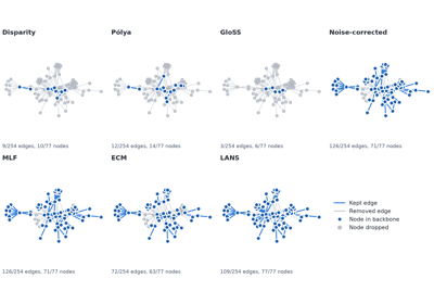
Method gallery
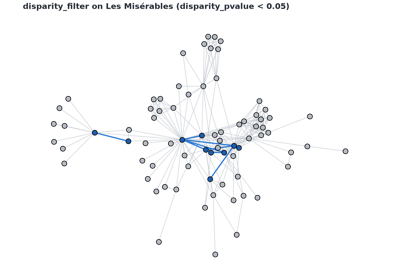
disparity_filter() on Les Misérables, keeping disparity_pvalue < 0.05.
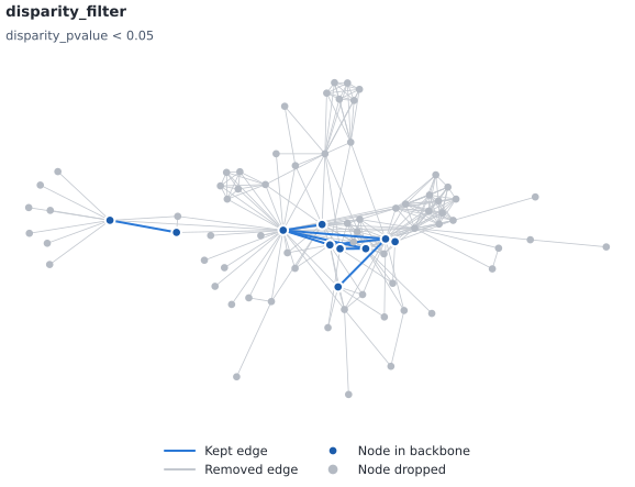
Backbone (blue) over the original graph (gray). Kept 9 of 254 edges (4%) and 10 of 77 nodes.#
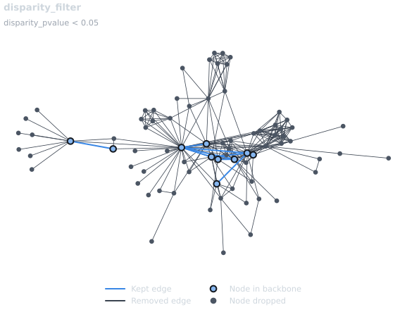
Backbone (blue) over the original graph (gray). Kept 9 of 254 edges (4%) and 10 of 77 nodes.#
noise_corrected_filter() on Les Misérables, keeping nc_pvalue < 0.05.
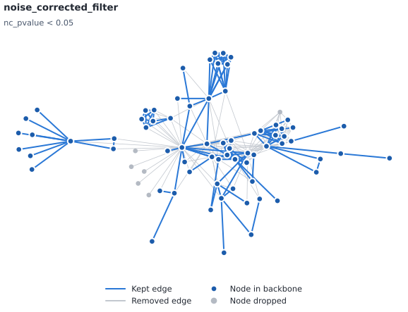
Backbone (blue) over the original graph (gray). Kept 126 of 254 edges (50%) and 71 of 77 nodes.#
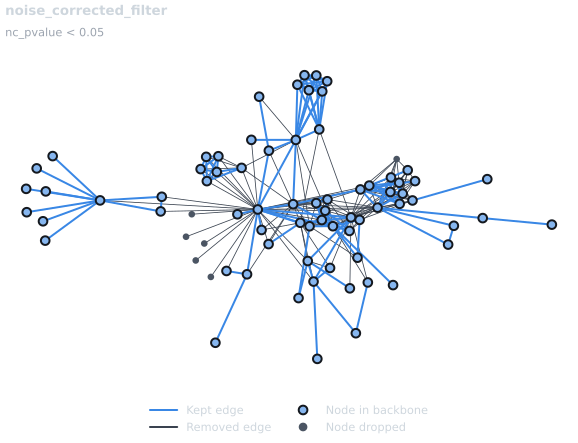
Backbone (blue) over the original graph (gray). Kept 126 of 254 edges (50%) and 71 of 77 nodes.#
marginal_likelihood_filter() on Les Misérables, keeping ml_pvalue < 0.05.
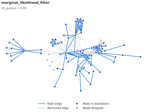
Backbone (blue) over the original graph (gray). Kept 126 of 254 edges (50%) and 71 of 77 nodes.#
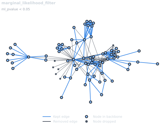
Backbone (blue) over the original graph (gray). Kept 126 of 254 edges (50%) and 71 of 77 nodes.#
ecm_filter() on Les Misérables, keeping ecm_pvalue < 0.05.
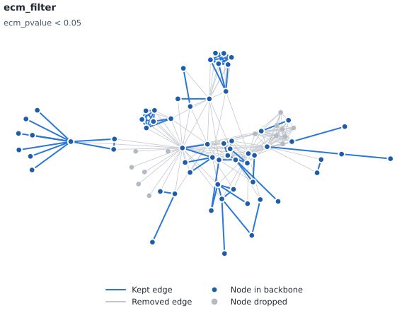
Backbone (blue) over the original graph (gray). Kept 72 of 254 edges (28%) and 63 of 77 nodes.#
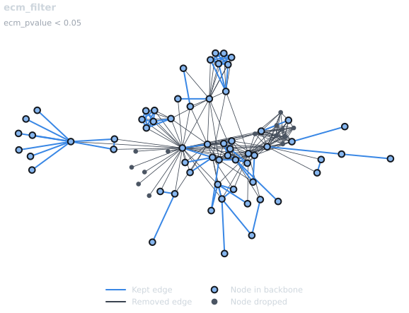
Backbone (blue) over the original graph (gray). Kept 72 of 254 edges (28%) and 63 of 77 nodes.#
lans_filter() on Les Misérables, keeping lans_pvalue < 0.05.
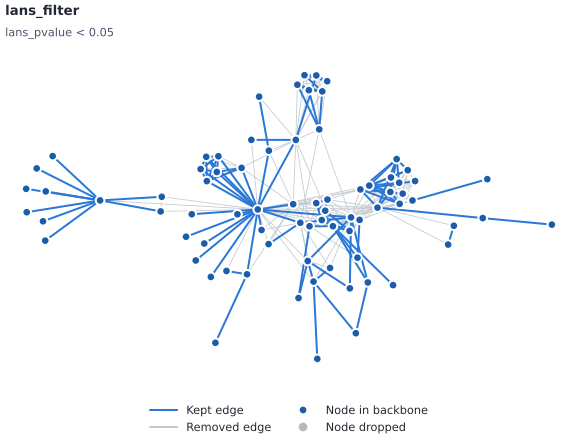
Backbone (blue) over the original graph (gray). Kept 109 of 254 edges (43%) and 77 of 77 nodes.#
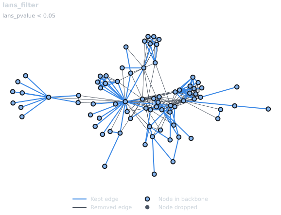
Backbone (blue) over the original graph (gray). Kept 109 of 254 edges (43%) and 77 of 77 nodes.#
multiple_linkage_analysis() on Les Misérables, keeping mla_keep.
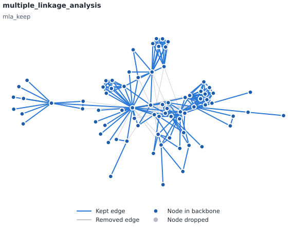
Backbone (blue) over the original graph (gray). Kept 205 of 254 edges (81%) and 77 of 77 nodes.#
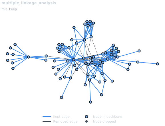
Backbone (blue) over the original graph (gray). Kept 205 of 254 edges (81%) and 77 of 77 nodes.#
polya_filter() on Les Misérables, keeping polya_pvalue < 0.05.
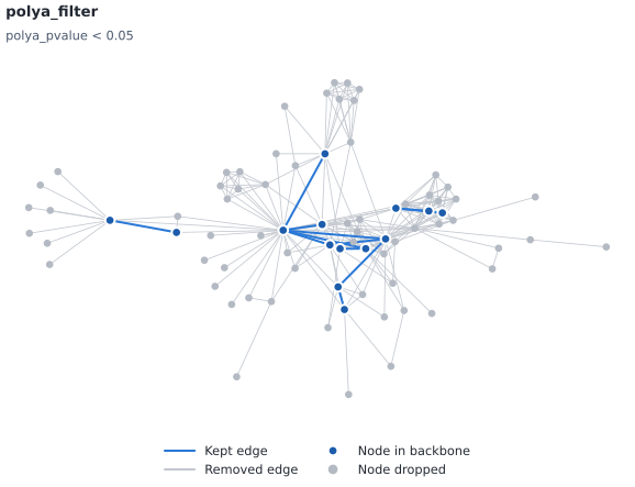
Backbone (blue) over the original graph (gray). Kept 12 of 254 edges (5%) and 14 of 77 nodes.#
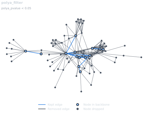
Backbone (blue) over the original graph (gray). Kept 12 of 254 edges (5%) and 14 of 77 nodes.#
gloss_filter() on Les Misérables, keeping gloss_pvalue < 0.05.
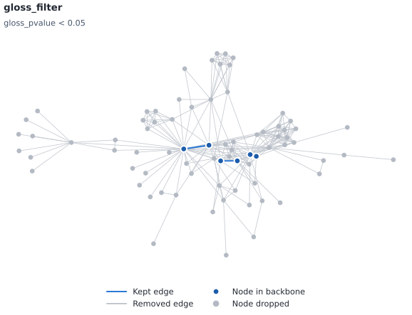
Backbone (blue) over the original graph (gray). Kept 3 of 254 edges (1%) and 6 of 77 nodes.#
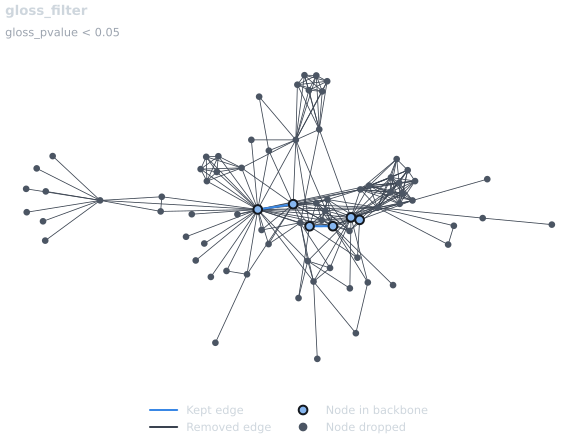
Backbone (blue) over the original graph (gray). Kept 3 of 254 edges (1%) and 6 of 77 nodes.#
Alias Names
- nx_backbone.disparity(G, weight='weight', signed=False, missing_as_zero=False, a=1.0)[source]#
Alias for
disparity_filter().Computational complexity estimate is
O(n + m)time andO(n + m)space.
- nx_backbone.mlf(G, weight='weight', signed=False, missing_as_zero=False, unit=1)[source]#
Alias for
marginal_likelihood_filter().Computational complexity estimate is
O(n + m)time andO(n + m)space.
- nx_backbone.lans(G, weight='weight', signed=False, missing_as_zero=False)[source]#
Alias for
lans_filter().Computational complexity estimate is
O(m log n)time andO(n + m)space.