From a hairball to a backbone, end to end

Draw a weighted network with a few hundred edges and you get a hairball: a tangle in which every node seems tied to every other and no structure stands out. A backbone is a subgraph that keeps the edges that carry the network’s structure and drops the rest, so that the structure can be seen and, more importantly, analyzed.

This page is a worked case study of the whole process, from the first plot to the methods paragraph of a paper. Each step says why it is needed before showing how:

1. why a single weight cut is not enough;

2. how scoring an edge differs from filtering it;

3. how to choose a significance level and correct for running one test per edge;

4. how to compare backbones from different methods;

5. how to check that a backbone is robust, and what it preserves;

6. how to report it.

It assumes you have read the Quick Start. The short how-to pages in Tutorials cover each method in more detail, and this page links to them along the way. Every number and figure below is computed when the documentation is built, so the text always matches the code.

Setup

Besides networkx and nx_backbone, this page uses NumPy, SciPy (for the marginal likelihood filter) and Matplotlib; pip install "nx-backbone[full,viz]" installs them all.

The figures use the documentation’s shared figure style, docs/_figures/style.py in the repository: its colors, a fixed layout per network, and draw_backbone(), which draws a backbone over the original graph. Each figure is drawn by a function of the color mode ("light" or "dark") so that the page can show the version that matches your theme; show saves both. In your own notebook, call the drawing function and Matplotlib shows the figure.

import tempfile
from collections import Counter
from pathlib import Path

import matplotlib.patheffects as pe
import matplotlib.pyplot as plt
import networkx as nx
import numpy as np
from _figures import style
from matplotlib.cm import ScalarMappable
from matplotlib.collections import LineCollection
from matplotlib.colors import Normalize
from matplotlib.lines import Line2D

import nx_backbone as nb



def show(draw, name, fmt="svg"):
    """Save a light and a dark version of the figure that ``draw(mode)`` makes.

    Drawings of the larger network, with thousands of edges, are saved as PNG
    rather than SVG to keep the page light.
    """
    style.save_variants(
        draw, IMAGES / name, fmt=fmt, **({"dpi": 120} if fmt == "png" else {})
    )

Two networks

The case study follows two weighted networks. In both, an edge’s weight counts how often two nodes were seen together.

Les Misérables is the co-appearance network of the characters of Victor Hugo’s novel (Knuth, 1993), bundled with NetworkX: two characters are linked when they appear in the same chapter, weighted by how often they do. It is small, and every node has a name, which makes it good for building intuition.

A simulated collaboration network stands in for the larger networks of real studies. Researchers belong to four departments and are more likely to work with colleagues in their own department. Each researcher also has an activity level, drawn from a heavy-tailed (lognormal) distribution, so a few are prolific and most are not. A tie’s weight, the number of joint papers, grows with both researchers’ activity, is larger within a department, and is noisy. Because the network is simulated, we know the departments: the structure a good backbone should reveal.

def collaboration_network(
    n_departments=4, size=50, p_within=0.4, p_between=0.06, boost=8, seed=7
):
    """A seeded weighted network with planted departments (node attribute "block")."""
    rng = np.random.default_rng(seed)
    p = [
        [p_within if i == j else p_between for j in range(n_departments)]
        for i in range(n_departments)
    ]
    G = nx.stochastic_block_model([size] * n_departments, p, seed=seed)
    activity = rng.lognormal(0.0, 1.0, G.number_of_nodes())
    for u, v, data in G.edges(data=True):
        same = G.nodes[u]["block"] == G.nodes[v]["block"]
        rate = activity[u] * activity[v] * (boost if same else 1)
        data["weight"] = int(np.ceil(rate * rng.lognormal(0.0, 1.5)))
    return G


L = nx.les_miserables_graph()
S = collaboration_network()
DEPARTMENT = nx.get_node_attributes(S, "block")
NETWORKS = {"Les Misérables": L, "Collaborations": S}

print(f"{'network':<16} {'nodes':>5} {'edges':>5} {'weights':>9} {'degrees':>8}")
for name, G in NETWORKS.items():
    w = [w for _, _, w in G.edges(data="weight")]
    k = [k for _, k in G.degree()]
    print(
        f"{name:<16} {G.number_of_nodes():>5} {G.number_of_edges():>5} "
        f"{min(w):>4}-{max(w):<4} {min(k):>4}-{max(k):<3}"
    )

network          nodes edges   weights  degrees
Les Misérables      77   254    1-31      1-36
Collaborations     200  2757    1-2142   16-41

1. The problem: a hairball

Here are both networks drawn in full. Every edge is drawn, and the collaboration network in particular is a solid tangle: you cannot see the departments, let alone who works with whom.

pos_L = style.layout(L, "les_miserables")
pos_S = style.layout(S, "collaboration_network")
CENTERS = {
    d: np.mean([pos_S[n] for n in S if DEPARTMENT[n] == d], axis=0)
    for d in sorted(set(DEPARTMENT.values()))
}


def label_departments(ax, mode):
    """Name each department just outside its cluster of nodes."""
    pal = style.palette(mode)
    halo = [pe.withStroke(linewidth=3, foreground=pal.surface)]
    for d, center in CENTERS.items():
        r = np.linalg.norm(center)
        x, y = center * (r + 0.6) / r
        ax.text(
            x,
            y,
            f"Dept. {'ABCD'[d]}",
            ha="center",
            va="center",
            fontsize=8.5,
            fontweight="bold",
            color=pal.muted,
            path_effects=halo,
        )


def draw_hairballs(mode):
    fig, axes = plt.subplots(1, 2, figsize=(8, 4.2))
    panels = [(axes[0], L, pos_L, 30.0), (axes[1], S, pos_S, 14.0)]
    for (ax, G, pos, size), name in zip(panels, NETWORKS):
        style.draw_backbone(
            ax, G, G, pos, mode=mode, legend=False, node_size=size, kept_width=0.5
        )
        ax.set_title(f"{name}: {G.number_of_edges()} edges")
        ax.set_anchor("N")
    return fig


show(draw_hairballs, "hairballs", fmt="png")

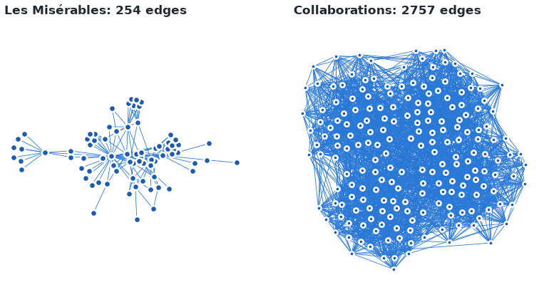
Both networks drawn in full, every edge in the same color. The edge counts are in the panel titles.

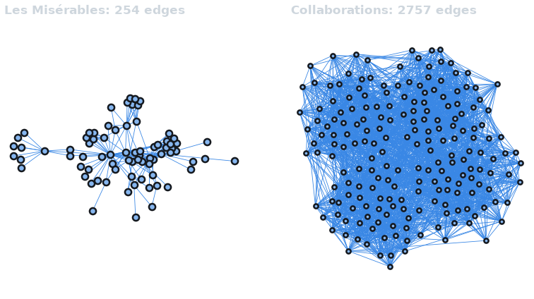
Both networks drawn in full, every edge in the same color. The edge counts are in the panel titles.

The obvious fix is a global weight cut: keep the edges whose weight is at least some threshold t and drop the rest. To see why it fails, look at how the weights are spread. Two quantities matter: a node’s degree, its number of edges, and its strength, the sum of its edges’ weights.

def weights(G):
    return np.array([w for _, _, w in G.edges(data="weight")])


def global_cut_curve(G):
    """Share of edges kept, and of nodes left with an edge, at every weight cut."""
    w = weights(G)
    edges = list(G.edges())
    rows = []
    for t in np.unique(w):
        kept = [e for e, we in zip(edges, w) if we >= t]
        nodes = {n for e in kept for n in e}
        rows.append((len(kept) / len(edges), len(nodes) / G.number_of_nodes()))
    return np.array(rows)


def draw_distributions(mode):
    pal = style.palette(mode)
    colors = style.categorical(2, mode)
    marks = [("o", "-"), ("^", "--")]
    fig, axes = plt.subplots(1, 3, figsize=(9.5, 3.4), layout="constrained")
    for (name, G), color, (marker, ls) in zip(NETWORKS.items(), colors, marks):
        w = np.sort(weights(G))
        share = 1.0 - np.arange(len(w)) / len(w)
        axes[0].step(w, share, where="post", color=color, ls=ls, label=name)
        degree = [G.degree(n) for n in G]
        strength = [G.degree(n, weight="weight") for n in G]
        axes[1].scatter(
            degree,
            strength,
            s=16,
            marker=marker,
            color=color,
            edgecolors=pal.surface,
            linewidths=0.5,
        )
        curve = global_cut_curve(G)
        axes[2].plot(curve[:, 0], curve[:, 1], color=color, ls=ls)
    axes[0].set(
        xscale="log",
        yscale="log",
        xlabel="Edge weight w",
        ylabel="Share of edges with weight ≥ w",
        title="a. Weights span decades",
    )
    axes[1].set(
        xscale="log",
        yscale="log",
        xlabel="Degree (number of edges)",
        ylabel="Strength (total weight)",
        title="b. Same degree, unequal strength",
    )
    axes[2].set(
        xscale="log",
        xlabel="Share of edges kept by the cut",
        ylabel="Share of nodes left with an edge",
        ylim=(0, 1.04),
        title="c. A global cut drops nodes",
    )
    for ax in axes:
        ax.grid(True, which="major")
    handles = [
        Line2D([], [], color=c, ls=ls, marker=m, markersize=5, label=name)
        for name, c, (m, ls) in zip(NETWORKS, colors, marks)
    ]
    fig.legend(handles=handles, loc="outside upper center", ncols=2)
    return fig


show(draw_distributions, "distributions")

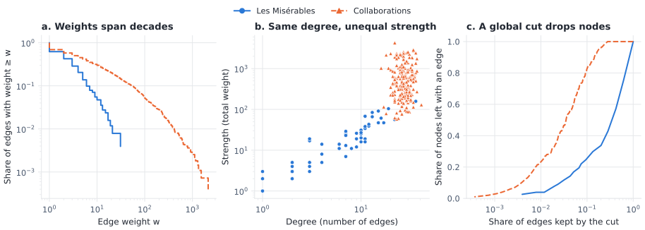
(a) Edge weights are heavy-tailed. (b) Nodes with the same number of edges differ greatly in total weight. (c) As a global weight cut gets stricter, whole nodes lose every edge. Solid lines and circles: Les Misérables; dashed lines and triangles: collaborations.

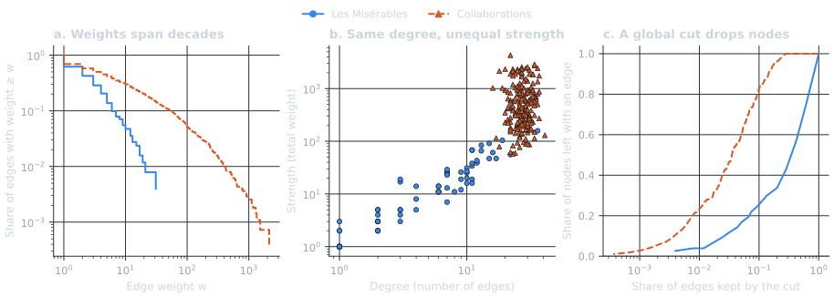
(a) Edge weights are heavy-tailed. (b) Nodes with the same number of edges differ greatly in total weight. (c) As a global weight cut gets stricter, whole nodes lose every edge. Solid lines and circles: Les Misérables; dashed lines and triangles: collaborations.

Panel (b) is the heart of the problem. A tie of a given weight is everything to a node of small strength and noise to a node of large strength, so no single threshold suits both. A cut strict enough to thin out the busy nodes removes every tie of the quiet ones, and they vanish from the backbone (panel c). Serrano, Boguñá and Vespignani (2009) call networks like this multiscale: the important ties live at different scales in different parts of the network.

Here is the cut at the 90th percentile of the weights, scored with global_threshold_filter() and filtered with boolean_filter():

for name, G in NETWORKS.items():
    t = np.quantile(weights(G), 0.9)
    cut = nb.boolean_filter(nb.global_threshold_filter(G, t), "global_threshold_keep")
    print(
        f"{name}: weight >= {t:g} keeps {nb.edge_fraction(G, cut):.0%} of the "
        f"edges but leaves only {nb.node_fraction(G, cut):.0%} of the nodes "
        "with an edge"
    )

Les Misérables: weight >= 6 keeps 13% of the edges but leaves only 30% of the nodes with an edge
Collaborations: weight >= 53 keeps 10% of the edges but leaves only 83% of the nodes with an edge

What we want instead is a rule that judges each edge against what is normal for its own endpoints. That needs a model of what “normal” means.

2. Scoring versus filtering

Every method in nx_backbone works in two steps (see Workflow):

• a scorer returns a copy of the graph with a score on every edge, here a p-value;

• a filter, such as threshold_filter(), keeps the edges whose score passes a rule.

Keeping the two apart means you score once and can then try, compare and report different rules without recomputing anything.

The scorer we start with is the disparity filter (Serrano et al., 2009). It asks, for each node, whether the node’s weight is concentrated on some of its edges more than chance would produce. The chance model, or null model, says that a node of degree k and strength s splits its strength over its k edges at random (formally, at k - 1 uniformly random cut points). Under that null, the share \(x = w / s\) that one edge gets is at least \(x\) with probability

\[p = (1 - x)^{k - 1}.\]

That probability is the edge’s p-value from this endpoint: how surprising its share would be if the node spread its strength at random. A small p-value means the edge is unusually strong for this node, whatever the node’s own scale. Each edge is tested from both endpoints, and its p-value is the smaller of the two, so an edge is kept when it matters to either of the nodes it joins.

scored_L = nb.disparity_filter(L)
pvalues_L = {(u, v): p for u, v, p in scored_L.edges(data="disparity_pvalue")}
for (u, v), p in sorted(pvalues_L.items(), key=lambda item: item[1])[:5]:
    print(f"{u:>12} - {v:<12} weight {L[u][v]['weight']:>2}  p = {p:.4f}")

     Valjean - Cosette      weight 31  p = 0.0005
     Valjean - Javert       weight 17  p = 0.0008
MmeThenardier - Thenardier   weight 13  p = 0.0081
     Valjean - Marius       weight 19  p = 0.0113
     Cosette - Marius       weight 21  p = 0.0173

The map below colors each edge by the strength of its evidence, \(-\log_{10} p\), so that an edge with \(p = 0.001\) scores 3 and an edge with \(p = 1\) scores 0. Stronger evidence is drawn thicker as well as in a stronger color.

evidence_L = {e: -np.log10(p) for e, p in pvalues_L.items()}
LABELED = ["Valjean", "Fauchelevent", "Cosette", "Myriel"]


def draw_pvalue_map(mode):
    pal = style.palette(mode)
    cmap = style.sequential_cmap(mode)
    norm = Normalize(0, max(evidence_L.values()))
    fig, ax = plt.subplots(figsize=(7.5, 5.2), layout="constrained")
    edges = sorted(evidence_L, key=evidence_L.get)  # strongest drawn on top
    ax.add_collection(
        LineCollection(
            [(pos_L[u], pos_L[v]) for u, v in edges],
            colors=[cmap(norm(evidence_L[e])) for e in edges],
            linewidths=[0.4 + 2.6 * norm(evidence_L[e]) for e in edges],
            capstyle="round",
        )
    )
    xy = np.array([pos_L[n] for n in L])
    ax.scatter(*xy.T, s=22, c=pal.node, edgecolors=pal.surface, linewidths=1, zorder=3)
    halo = [pe.withStroke(linewidth=3, foreground=pal.surface)]
    for name in LABELED:
        x, y = pos_L[name]
        ax.annotate(
            name,
            (x, y),
            xytext=(5, 5),
            textcoords="offset points",
            fontsize=8.5,
            color=pal.ink,
            path_effects=halo,
            zorder=4,
        )
    ax.set_aspect("equal")
    ax.autoscale_view()
    ax.set_axis_off()
    cbar = fig.colorbar(ScalarMappable(norm, cmap), ax=ax, shrink=0.7, pad=0.02)
    cbar.set_label("Evidence (p-value, log scale)")
    cbar.outline.set_visible(False)
    level = -np.log10(0.05)
    cbar.ax.axhline(level, color=pal.ink, lw=1.2)
    ticks = [0, level, 2, 3]
    cbar.set_ticks(ticks, labels=["p = 1", "p = 0.05", "p = 0.01", "p = 0.001"])
    ax.set_title("Disparity-filter evidence on Les Misérables")
    return fig


show(draw_pvalue_map, "pvalue_map")

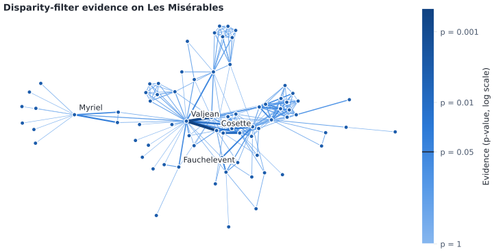
Disparity-filter evidence, \(-\log_{10} p\), for every edge of Les Misérables. Darker and thicker means stronger evidence; the mark on the color bar is \(p = 0.05\).

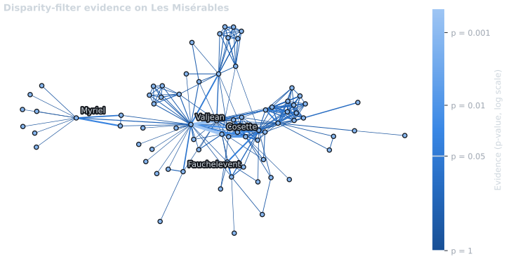
Disparity-filter evidence, \(-\log_{10} p\), for every edge of Les Misérables. Brighter and thicker means stronger evidence; the mark on the color bar is \(p = 0.05\).

Most edges carry little evidence. To see why, look at the test from two endpoints: Valjean, the hero, who has the most ties in the novel, and Fauchelevent, who has only a few, most of his weight going to Valjean.

def endpoint_tests(G, node):
    """Weight share and one-endpoint p-value of each of *node*'s edges."""
    k = G.degree(node)
    s = G.degree(node, weight="weight")
    return {
        nbr: (d["weight"] / s, (1 - d["weight"] / s) ** (k - 1))
        for nbr, d in G[node].items()
    }


FOCUS = ["Valjean", "Fauchelevent"]
tests = {node: endpoint_tests(L, node) for node in FOCUS}
for node in FOCUS:
    k = L.degree(node)
    needed = 1 - 0.05 ** (1 / (k - 1))
    nbr, (x, p) = max(tests[node].items(), key=lambda item: item[1][0])
    print(
        f"{node}: {k} edges. Largest share {x:.0%} (to {nbr}), p = {p:.4f}. "
        f"A share of at least {needed:.0%} is needed for p < 0.05."
    )
k_median = np.median([k for _, k in L.degree()])
print(
    f"Median degree in Les Misérables: {k_median:g}, so a typical character "
    f"needs a share of at least {1 - 0.05 ** (1 / (k_median - 1)):.0%} for p < 0.05."
)



def draw_null(mode):
    pal = style.palette(mode)
    fig, axes = plt.subplots(1, 2, figsize=(8.5, 3.4), layout="constrained")
    x = np.linspace(0, 1, 400)[:-1]
    halo = [pe.withStroke(linewidth=3, foreground=pal.surface)]
    for ax, node in zip(axes, FOCUS):
        k = L.degree(node)
        ax.plot(x, (1 - x) ** (k - 1), color=pal.muted, lw=1.2)
        ax.axhline(0.05, color=pal.ink, lw=0.8)
        ax.text(
            0.99,
            0.05 * 1.25,
            "p = 0.05",
            ha="right",
            va="bottom",
            fontsize=8,
            color=pal.ink,
            transform=ax.get_yaxis_transform(),
        )
        shares = np.array(list(tests[node].values()))
        sig = shares[:, 1] < 0.05
        ax.scatter(
            *shares[~sig].T,
            s=30,
            facecolors="none",
            edgecolors=pal.muted,
            linewidths=1.2,
            zorder=3,
            label="Not significant",
        )
        ax.scatter(
            *shares[sig].T,
            s=34,
            color=pal.kept,
            edgecolors=pal.surface,
            linewidths=1,
            zorder=4,
            label="Significant from this end",
        )
        nbr, (xs, ps) = max(tests[node].items(), key=lambda item: item[1][0])
        ax.annotate(
            f"{nbr}, p = {ps:.2g}",
            (xs, ps),
            xytext=(8, 6),
            textcoords="offset points",
            fontsize=8.5,
            color=pal.ink,
            path_effects=halo,
        )
        ax.set(
            yscale="log",
            ylim=(2e-4, 1.6),
            xlim=(0, 1),
            xlabel=f"Share of {node}'s strength on one edge",
            ylabel="p-value under the null",
            title=f"{node}: {k} edges",
        )
        ax.grid(True)
    axes[0].legend(loc="upper right")
    return fig


show(draw_null, "null_model")

Valjean: 36 edges. Largest share 20% (to Cosette), p = 0.0005. A share of at least 8% is needed for p < 0.05.
Fauchelevent: 4 edges. Largest share 57% (to Valjean), p = 0.0787. A share of at least 63% is needed for p < 0.05.
Median degree in Les Misérables: 6, so a typical character needs a share of at least 45% for p < 0.05.

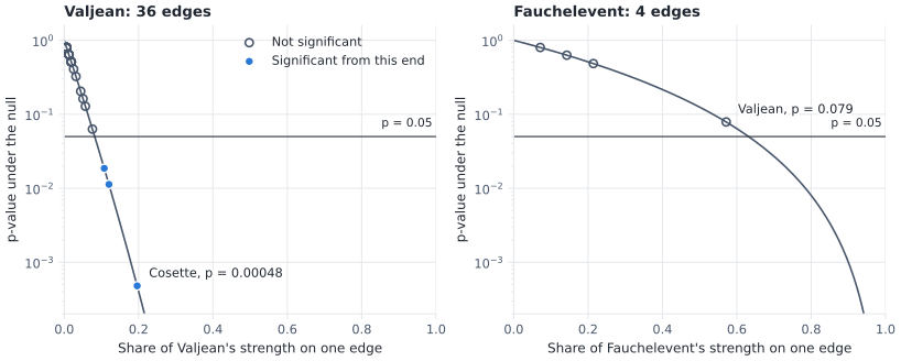
The disparity filter’s test from one endpoint. The curve is the p-value the null model gives each possible weight share; the points are the node’s actual edges, filled when they pass \(p < 0.05\). With many edges (left), a modest share is already surprising; with few edges (right), even a majority share is not.

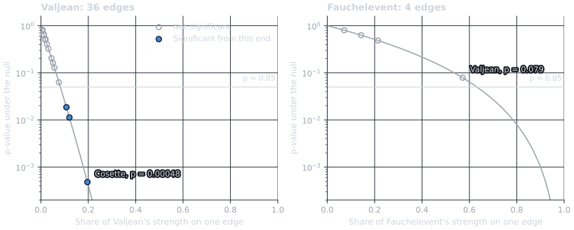
The disparity filter’s test from one endpoint. The curve is the p-value the null model gives each possible weight share; the points are the node’s actual edges, filled when they pass \(p < 0.05\). With many edges (left), a modest share is already surprising; with few edges (right), even a majority share is not.

This is the price of a local null model. Each node is judged on its own scale, which is what rescues the quiet nodes from the global cut, but a node with few edges offers little evidence either way: with only a few random cut points, a lopsided split happens by chance quite often. As the last line printed above shows, a typical Les Misérables character must give a single tie a large part of their weight before the test notices.

Now the filtering step: keep the edges with \(p < 0.05\).

backbone_L = nb.threshold_filter(scored_L, "disparity_pvalue", 0.05)
print(f"Kept {backbone_L.number_of_edges()} of {L.number_of_edges()} edges.")

Kept 9 of 254 edges.

A small backbone. Is it a real finding? That depends on how many edges would pass by chance, which is the next question.

3. Choosing alpha and correcting for multiple tests

The threshold 0.05 is the significance level, \(\alpha\): the probability of keeping an edge that is no stronger than the null model predicts. That is a fair risk for a single test, but a backbone runs one test per edge. With m edges, about \(\alpha m\) of them pass by chance even if none is truly strong.

A multiple-testing correction adjusts the p-values for the number of tests before they are compared with \(\alpha\). Two kinds matter:

• the Bonferroni correction multiplies each p-value by m. It controls the family-wise error rate: the probability of keeping even one false edge. Holm’s (1979) step-down version is never less powerful;

• the Benjamini-Hochberg (BH) procedure (Benjamini & Hochberg, 1995) controls the false discovery rate: the expected share of false edges among those kept. It keeps more edges, at the cost of a controlled share of mistakes.

threshold_filter() applies either with its mtc argument; adjust_pvalues() returns the adjusted values themselves. Below, the number of edges each rule keeps is traced over a range of \(\alpha\), for both networks.

scored_S = nb.disparity_filter(S)
CORRECTIONS = {"none": "No correction", "bonferroni": "Bonferroni", "bh": "BH"}
ALPHAS = np.logspace(-4, np.log10(0.5), 120)


def kept_by_alpha(scored, alphas=ALPHAS):
    """Edges kept at each alpha, for each correction: counts of adjusted p < alpha."""
    p = [p for _, _, p in scored.edges(data="disparity_pvalue")]
    return {
        mtc: np.searchsorted(
            np.sort(p if mtc == "none" else nb.adjust_pvalues(p, mtc)), alphas
        )
        for mtc in CORRECTIONS
    }


curves = {
    "Les Misérables": kept_by_alpha(scored_L),
    "Collaborations": kept_by_alpha(scored_S),
}
print(
    f"{'network':<16} {'alpha':>5} "
    + " ".join(f"{c:>13}" for c in CORRECTIONS.values())
)
for name, scored in [("Les Misérables", scored_L), ("Collaborations", scored_S)]:
    for alpha in (0.01, 0.05, 0.1):
        counts = [
            nb.threshold_filter(
                scored, "disparity_pvalue", alpha, mtc=mtc
            ).number_of_edges()
            for mtc in CORRECTIONS
        ]
        print(f"{name:<16} {alpha:>5} " + " ".join(f"{c:>13}" for c in counts))
    m = scored.number_of_edges()
    print(f"{'':<16} expected to pass by chance at alpha = 0.05: about {0.05 * m:.0f}")



def draw_alpha_curves(mode):
    pal = style.palette(mode)
    colors = style.categorical(3, mode)
    styles = ["-", "--", ":"]
    fig, axes = plt.subplots(1, 2, figsize=(8.5, 3.5), layout="constrained")
    for ax, (name, curve) in zip(axes, curves.items()):
        for (mtc, label), color, ls in zip(CORRECTIONS.items(), colors, styles):
            ax.step(ALPHAS, curve[mtc], where="post", color=color, ls=ls, label=label)
        ax.axvline(0.05, color=pal.ink, lw=0.8)
        ax.text(
            0.05 * 1.1,
            0.97,
            "α = 0.05",
            transform=ax.get_xaxis_transform(),
            fontsize=8,
            color=pal.ink,
            va="top",
        )
        ax.set(
            xscale="log", xlabel="Significance level α", ylabel="Edges kept", title=name
        )
        ax.set_ylim(bottom=0)
        ax.grid(True)
    fig.legend(
        *axes[0].get_legend_handles_labels(), loc="outside upper center", ncols=3
    )
    return fig


show(draw_alpha_curves, "alpha_curves")

network          alpha No correction    Bonferroni            BH
Les Misérables    0.01             3             0             0
Les Misérables    0.05             9             0             0
Les Misérables     0.1            21             0             2
                 expected to pass by chance at alpha = 0.05: about 13
Collaborations    0.01           238            69           131
Collaborations    0.05           348            84           194
Collaborations     0.1           433            90           231
                 expected to pass by chance at alpha = 0.05: about 138

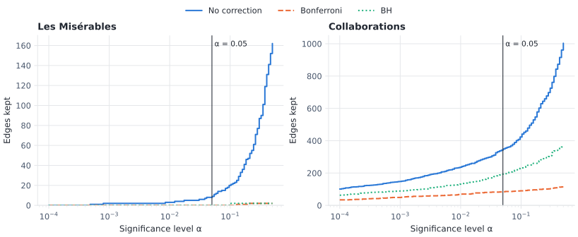
Edges kept as \(\alpha\) grows, with no correction (solid), Bonferroni (dashed) and Benjamini-Hochberg (dotted). The vertical line marks \(\alpha = 0.05\); the table above gives the values at three levels.

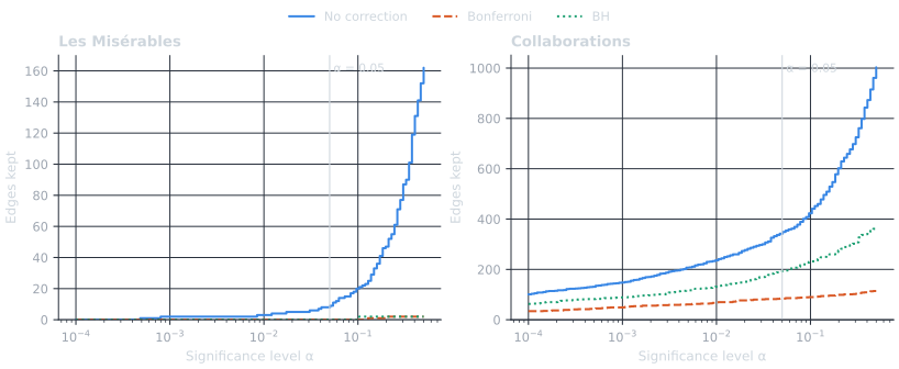
Edges kept as \(\alpha\) grows, with no correction (solid), Bonferroni (dashed) and Benjamini-Hochberg (dotted). The vertical line marks \(\alpha = 0.05\); the table above gives the values at three levels.

The two networks tell different stories:

• Les Misérables. The uncorrected backbone is no larger than the number of edges expected to pass by chance, and no edge survives either correction at \(\alpha = 0.05\). With so many low-degree nodes, the disparity filter has too little power (ability to detect a truly strong edge) here, and its backbone should not be reported as a set of significant ties. Validating a Backbone shows that a method with more power on this network, the marginal likelihood filter, does keep edges after correction.

• Collaborations. With more edges per node, the tests have power, and the corrections trim the backbone rather than empty it.

One more caution: because an edge’s p-value is the smaller of its two endpoint tests, the disparity filter passes somewhat more than a share \(\alpha\) of edges when the null model holds (see the Notes of disparity_filter()). A correction guards against that too.

From here on we follow the collaboration network with BH at \(\alpha = 0.05\): the backbone is meant to describe the network’s overall structure, where a small, controlled share of false edges is acceptable. Choose the correction and \(\alpha\) before looking at the result, and report both.

backbone = nb.threshold_filter(scored_S, "disparity_pvalue", 0.05, mtc="bh")

The payoff: local beats global

Is the disparity backbone better than a global cut of the same size? Pick the weight threshold that keeps about as many edges (ties at the threshold can add a few more) and compare.

k = backbone.number_of_edges()
t = np.sort(weights(S))[::-1][k - 1]
global_cut = nb.boolean_filter(
    nb.global_threshold_filter(S, t), "global_threshold_keep"
)


def within_department(original, backbone):
    """Share of the backbone's edges that join two people in the same department."""
    edges = list(backbone.edges())
    return sum(DEPARTMENT[u] == DEPARTMENT[v] for u, v in edges) / len(edges)


for name, H in [("global cut", global_cut), ("disparity, BH", backbone)]:
    print(
        f"{name:<14} {H.number_of_edges():>4} edges, "
        f"{nb.node_fraction(S, H):.0%} of nodes with an edge, "
        f"{within_department(S, H):.0%} of edges within a department"
    )
print(f"(all edges: {within_department(S, S):.0%} within a department)")



def draw_global_vs_local(mode):
    fig, axes = plt.subplots(1, 2, figsize=(8, 4.6), layout="constrained")
    for ax, (title, H) in zip(
        axes, [("Global weight cut", global_cut), ("Disparity filter, BH", backbone)]
    ):
        counts = style.draw_backbone(
            ax, S, H, pos_S, mode=mode, legend=False, node_size=18
        )
        label_departments(ax, mode)
        ax.set_title(f"{title}\n{counts.short}")
    fig.legend(handles=style.legend_handles(mode), loc="outside lower center", ncols=4)
    return fig


show(draw_global_vs_local, "global_vs_local", fmt="png")

global cut      195 edges, 72% of nodes with an edge, 94% of edges within a department
disparity, BH   194 edges, 94% of nodes with an edge, 98% of edges within a department
(all edges: 68% within a department)

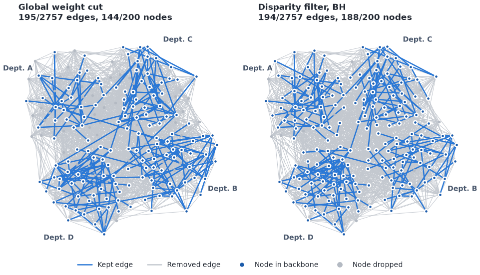
Two backbones of the collaboration network with about the same number of edges. Kept edges are blue over the removed edges in gray; nodes left without an edge are small and gray. The counts are in the panel titles.

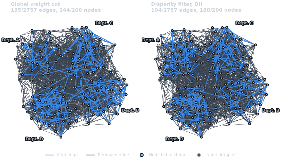
Two backbones of the collaboration network with about the same number of edges. Kept edges are blue over the removed edges in gray; nodes left without an edge are small and gray. The counts are in the panel titles.

With the same budget of edges, the global cut spends it on the ties among prolific researchers and leaves many people out entirely, while the disparity backbone keeps each researcher’s dominant ties, quiet or busy, and those ties are more often inside a department. That is the multiscale backbone of Serrano et al. (2009).

4. Comparing methods

The disparity filter is one answer to “which edges matter?”. Other methods ask the question differently, and a careful analysis tries more than one. Four families are worth comparing:

• Local null models judge each edge against its endpoints separately: the disparity filter.

• Global null models judge each edge against a model of the whole network. The marginal likelihood filter (Dianati, 2016) treats a weight as a count of unit edges whose two endpoints are drawn in proportion to the nodes’ strengths, and asks whether a pair co-occurs more often than that. Because it models the pair as a whole, a heavy edge can be significant even when it is a small share of each endpoint’s strength.

• Structural methods keep edges for the role they play in the network rather than for a test. The high-salience skeleton (Grady, Thiemann & Brockmann, 2012) treats \(1/w\) as a length, builds the tree of shortest paths from every node, and scores each edge by the share of these trees that use it; we keep edges used by at least half.

• Structural guarantees: the maximum spanning tree keeps the heaviest set of edges that still connects every node, so the backbone is connected by construction, with exactly one edge fewer than the number of nodes.

ml_S = nb.marginal_likelihood_filter(S)
backbones = {
    "Disparity filter": backbone,
    "Marginal likelihood": nb.threshold_filter(ml_S, "ml_pvalue", 0.05, mtc="bh"),
    "High-salience skeleton": nb.threshold_filter(
        nb.high_salience_skeleton(S), "salience", 0.5, mode="above"
    ),
    "Maximum spanning tree": nb.boolean_filter(
        nb.maximum_spanning_tree_backbone(S), "mst_keep"
    ),
}


def draw_small_multiples(mode):
    fig, axes = plt.subplots(2, 2, figsize=(8, 8.4), layout="constrained")
    for ax, (name, H) in zip(axes.flat, backbones.items()):
        counts = style.draw_backbone(
            ax, S, H, pos_S, mode=mode, legend=False, node_size=16
        )
        label_departments(ax, mode)
        ax.set_title(f"{name}\n{counts.short}")
    fig.legend(handles=style.legend_handles(mode), loc="outside lower center", ncols=4)
    return fig


show(draw_small_multiples, "small_multiples", fmt="png")

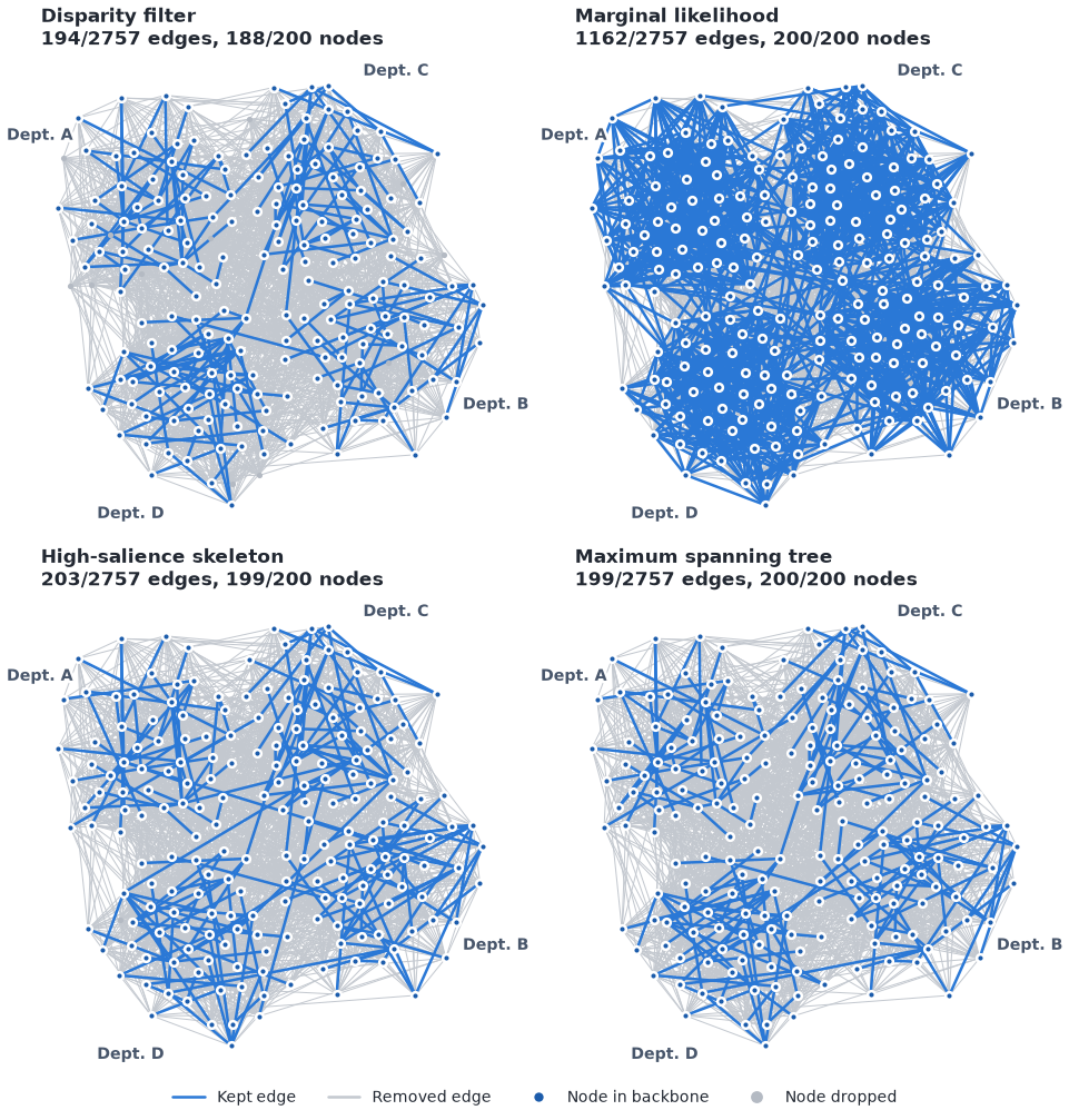
Four backbones of the collaboration network on one layout. Each panel title gives the method and how many edges and nodes it keeps.

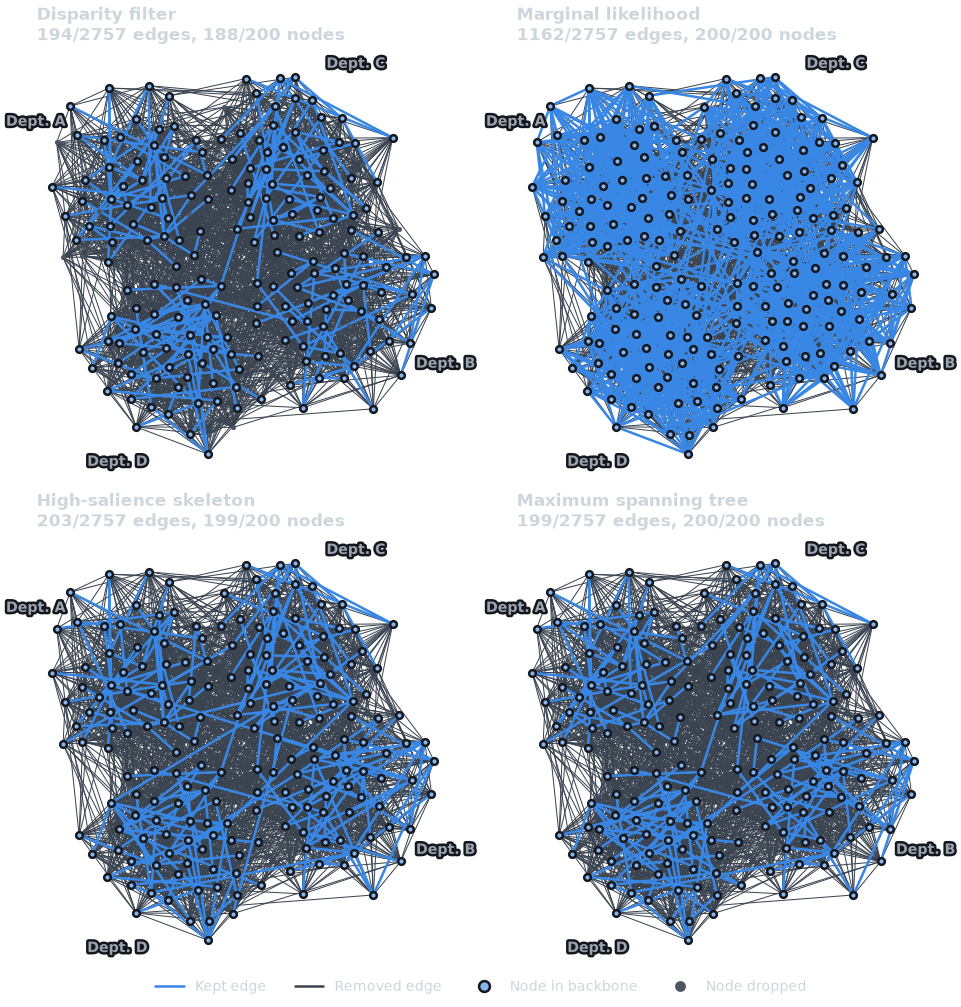
Four backbones of the collaboration network on one layout. Each panel title gives the method and how many edges and nodes it keeps.

Pictures invite over-reading, so put numbers beside them. compare_backbones() evaluates every backbone with any measure that takes (original, backbone): the shares of nodes, edges and total weight kept, the share of node pairs still joined by a path (reachability(), wrapped to take two arguments), and our own measure, the share of edges within a department.

def reachability(original, backbone):
    return nb.reachability(backbone)


measures = [
    nb.node_fraction,
    nb.edge_fraction,
    nb.weight_fraction,
    reachability,
    within_department,
]
results = nb.compare_backbones(S, backbones, measures=measures)
columns = ["nodes", "edges", "weight", "reach", "within"]
print(f"{'':<23}" + "".join(f"{c:>8}" for c in columns))
for name, row in results.items():
    print(f"{name:<23}" + "".join(f"{v:>8.2f}" for v in row.values()))


def within_edges(G):
    return {frozenset(e) for e in G.edges() if DEPARTMENT[e[0]] == DEPARTMENT[e[1]]}


ml_share = len(within_edges(backbones["Marginal likelihood"])) / len(within_edges(S))
print(
    f"The marginal likelihood backbone keeps {ml_share:.0%} of within-department ties."
)

                          nodes   edges  weight   reach  within
Disparity filter           0.94    0.07    0.61    0.60    0.98
Marginal likelihood        1.00    0.42    0.94    1.00    0.91
High-salience skeleton     0.99    0.07    0.61    0.91    0.95
Maximum spanning tree      1.00    0.07    0.62    1.00    0.96
The marginal likelihood backbone keeps 56% of within-department ties.

Reading the table:

• Sparsity and weight. A good backbone keeps few edges but much of the weight. Three of the four keep a similar small share of edges; the marginal likelihood filter keeps far more, because in a network with departments a large share of within-department ties is stronger than the strengths alone predict (printed above). Its null model answers a different question, not a worse one.

• Connectivity. The spanning tree joins every pair of nodes by construction. The disparity backbone, which has no structural guarantee, falls apart into pieces; the salience skeleton sits in between.

• Structure. Every backbone is more concentrated within departments than the original network, so each one sharpens the planted structure. Even the spanning tree, which must link the departments to each other, keeps mostly within-department edges.

No method wins on every column; the right one depends on what you will do with the backbone. Choosing a Method and Comparing Multiple Methods say more about the choice.

5. Validating

A backbone is a finding, so check it like one: does it change much when the analysis choices change, and does it keep what we care about?

Robustness to alpha

Backbones from one scorer at different levels of \(\alpha\) are nested: a stricter level keeps a subset of the edges. So the question is how much the size changes.

levels = {
    a: nb.threshold_filter(scored_S, "disparity_pvalue", a, mtc="bh")
    for a in (0.01, 0.05, 0.1)
}
for a, H in levels.items():
    print(
        f"alpha = {a:<5} {H.number_of_edges():>4} edges, "
        f"{nb.node_fraction(S, H):.0%} of nodes with an edge"
    )

alpha = 0.01   131 edges, 80% of nodes with an edge
alpha = 0.05   194 edges, 94% of nodes with an edge
alpha = 0.1    231 edges, 97% of nodes with an edge

Report the backbone together with that sensitivity, as in the table above, rather than as one number.

Robustness to the method

An edge that methods built on different ideas all keep is unlikely to be an artifact of any one of them. consensus_backbone() keeps the edges present in every backbone it is given; counting how many backbones keep each edge gives a graded answer instead of a yes or no.

core = nb.consensus_backbone(*backbones.values())
votes = Counter(frozenset(e) for H in backbones.values() for e in H.edges())
print(f"Kept by all {len(backbones)} methods: {core.number_of_edges()} edges")
for n_methods, n_edges in sorted(Counter(votes.values()).items()):
    print(f"  kept by {n_methods} of {len(backbones)} methods: {n_edges} edges")
singles = {e for e, v in votes.items() if v == 1}
for name, H in backbones.items():
    only = sum(frozenset(e) in singles for e in H.edges())
    print(f"  kept by {name} alone: {only} edges")



def draw_votes(mode):
    pal = style.palette(mode)
    ramp = pal.sequential[1:]  # four steps, low to high
    widths = [0.6, 1.0, 1.6, 2.4]
    fig, ax = plt.subplots(figsize=(7, 6.4), layout="constrained")
    removed = [e for e in S.edges() if frozenset(e) not in votes]
    ax.add_collection(
        LineCollection(
            [(pos_S[u], pos_S[v]) for u, v in removed],
            colors=pal.removed,
            linewidths=0.4,
            zorder=1,
        )
    )
    handles = []
    for n in range(1, len(backbones) + 1):
        edges = [tuple(e) for e, v in votes.items() if v == n]
        ax.add_collection(
            LineCollection(
                [(pos_S[u], pos_S[v]) for u, v in edges],
                colors=ramp[n - 1],
                linewidths=widths[n - 1],
                capstyle="round",
                zorder=1 + n,
            )
        )
        handles.append(
            Line2D(
                [],
                [],
                color=ramp[n - 1],
                lw=widths[n - 1],
                label=f"Kept by {n} of {len(backbones)}",
            )
        )
    xy = np.array([pos_S[n] for n in S])
    ax.scatter(
        *xy.T, s=12, c=pal.node, edgecolors=pal.surface, linewidths=0.8, zorder=8
    )
    handles.append(Line2D([], [], color=pal.removed, lw=1.5, label="Kept by none"))
    ax.set_aspect("equal")
    ax.autoscale_view()
    ax.set_axis_off()
    label_departments(ax, mode)
    ax.set_title("How many of the four backbones keep each edge")
    fig.legend(handles=handles, loc="outside lower center", ncols=5)
    return fig


show(draw_votes, "votes", fmt="png")

Kept by all 4 methods: 142 edges
  kept by 1 of 4 methods: 906 edges
  kept by 2 of 4 methods: 58 edges
  kept by 3 of 4 methods: 56 edges
  kept by 4 of 4 methods: 142 edges
  kept by Disparity filter alone: 0 edges
  kept by Marginal likelihood alone: 906 edges
  kept by High-salience skeleton alone: 0 edges
  kept by Maximum spanning tree alone: 0 edges

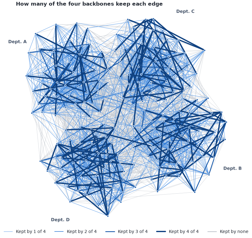
Agreement between the four backbones of section 4. Darker and thicker edges are kept by more methods; the counts are printed above.

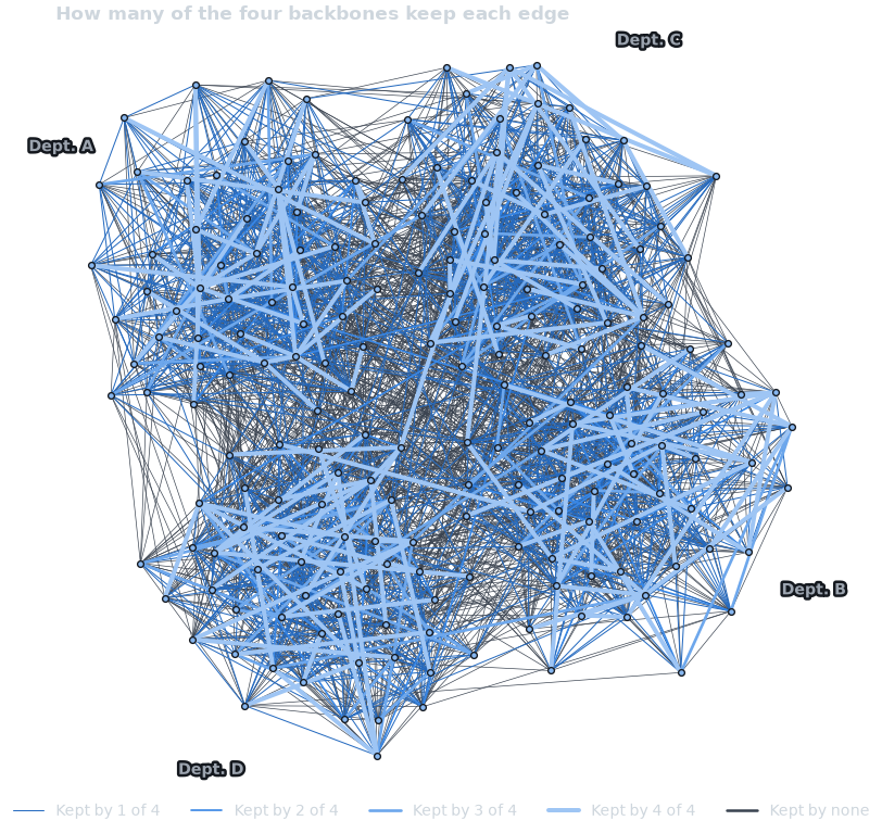
Agreement between the four backbones of section 4. Brighter and thicker edges are kept by more methods; the counts are printed above.

The edges every method keeps are the safest to interpret; edges kept by a single method deserve less weight. Here most of those come from the densest backbone, the marginal likelihood filter’s, which is another way of seeing that its null model asks a different question.

What the backbone preserves

The comparison table already answers part of this: the disparity backbone keeps a large share of the weight with few edges and concentrates on within-department ties, but it does not stay connected. Whether that matters depends on the analysis: for finding groups, a fragmented backbone that separates them is fine; for anything based on paths, such as distances or centralities, choose a method that keeps the network connected. Evaluating Backbones describes more measures, among them Kolmogorov-Smirnov distances between the degree and weight distributions of the original and the backbone.

A signed backbone

The tests so far are one-tailed: they look for edges that are stronger than the null model predicts. With signed=True, a scorer runs a two-tailed test, and an edge can also be significantly weaker than predicted. Each edge then gets a sign attribute: +1 for stronger, -1 for weaker. A negative edge records a tie that the null model expected and that did not happen, for example two prolific researchers who rarely work together.

signed = nb.marginal_likelihood_filter(S, signed=True)
signed_bb = nb.threshold_filter(signed, "ml_pvalue", 0.05, mtc="bh")
parts = {
    sign: signed_bb.edge_subgraph(
        (u, v) for u, v, s in signed_bb.edges(data="sign") if s == sign
    )
    for sign in (1, -1)
}
for sign, H in parts.items():
    label = "positive" if sign > 0 else "negative"
    print(
        f"{label}: {H.number_of_edges():>4} edges, "
        f"{within_department(S, H):.0%} within a department"
    )



def draw_signed(mode):
    fig, axes = plt.subplots(1, 2, figsize=(8, 4.7), layout="constrained")
    for ax, (sign, H) in zip(axes, parts.items()):
        style.draw_backbone(
            ax, S, H, pos_S, mode=mode, sign="sign", legend=False, node_size=16
        )
        label_departments(ax, mode)
        label = (
            "Positive: stronger than expected"
            if sign > 0
            else ("Negative: weaker than expected")
        )
        ax.set_title(f"{label}\n{H.number_of_edges()} edges")
    handles = style.legend_handles(mode, signed=True)[:3]
    fig.legend(handles=handles, loc="outside lower center", ncols=3)
    return fig


show(draw_signed, "signed", fmt="png")

positive: 1103 edges, 91% within a department
negative:   90 edges, 33% within a department

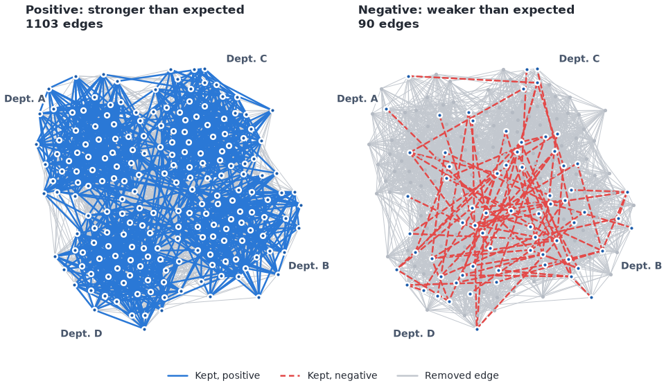
The signed marginal likelihood backbone (BH, \(\alpha = 0.05\)), split into its positive part (solid blue, left) and its negative part (dashed red, right). The counts are printed above.

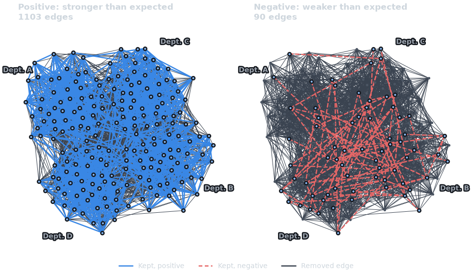
The signed marginal likelihood backbone (BH, \(\alpha = 0.05\)), split into its positive part (solid blue, left) and its negative part (dashed red, right). The counts are printed above.

The positive part looks like the department structure; the negative part points the other way, to ties that are rarer than the researchers’ activity predicts. Analyze the two parts separately: they answer different questions. Validating a Backbone shows a pitfall when splitting by sign (boolean_filter() treats -1 as true).

6. Reporting

A methods section should name the method and its null model, give \(\alpha\) and the correction, say how much of the network was kept and cite both the method and the software. describe_backbone() writes that paragraph from the same arguments you passed to the filter:

print(
    nb.describe_backbone(
        "disparity_filter", alpha=0.05, mtc="bh", original=S, backbone=backbone
    )
)

We extracted the backbone with the disparity filter (Serrano et al., 2009), which tests each edge's weight against a null model in which each node's strength is spread uniformly at random over its edges. Edges were kept if their p-value was below alpha = 0.05 after a Benjamini-Hochberg false discovery rate correction for multiple comparisons (Benjamini & Hochberg, 1995). The backbone retains 194 of 2757 edges (7.0%) and 188 of 200 non-isolated nodes (94.0%), and 61.4% of the total edge weight. Backbones were computed with nx-backbone version 0.3.0.post1.dev1 (Keegan, n.d.).

References

Benjamini, Y., & Hochberg, Y. (1995). Controlling the false discovery rate: a practical and powerful approach to multiple testing. Journal of the Royal Statistical Society: Series B, 57(1), 289-300.
Keegan, B. C. (n.d.). nx-backbone: Backbone extraction algorithms for complex networks (Version 0.3.0.post1.dev1) [Python package]. https://github.com/brianckeegan/nx-backbone
Serrano, M. A., Boguñá, M., & Vespignani, A. (2009). Extracting the multiscale backbone of complex weighted networks. Proceedings of the National Academy of Sciences, 106(16), 6483-6488. https://doi.org/10.1073/pnas.0808904106

style="bibtex" returns the same references as BibTeX entries for your reference manager:

print(nb.describe_backbone("disparity_filter", alpha=0.05, mtc="bh", style="bibtex"))

@article{serrano2009,
  author = {Serrano, M. A. and Boguñá, M. and Vespignani, A.},
  title = {Extracting the multiscale backbone of complex weighted networks},
  journal = {Proceedings of the National Academy of Sciences},
  volume = {106},
  number = {16},
  pages = {6483--6488},
  year = {2009},
  doi = {10.1073/pnas.0808904106}
}

@article{benjamini1995,
  author = {Benjamini, Y. and Hochberg, Y.},
  title = {Controlling the false discovery rate: a practical and powerful approach to multiple testing},
  journal = {Journal of the Royal Statistical Society: Series B},
  volume = {57},
  number = {1},
  pages = {289--300},
  year = {1995}
}

@misc{keegan_nx_backbone,
  author = {Keegan, Brian C.},
  title = {nx-backbone: Backbone extraction algorithms for complex networks},
  version = {0.3.0.post1.dev1},
  url = {https://github.com/brianckeegan/nx-backbone},
  note = {Python package}
}

Add the sensitivity analysis (the table of backbone sizes over \(\alpha\)) and the comparison with other methods, and the backbone is ready to report.

Where next

• The how-to pages. Statistical Backbone Extraction (every statistical scorer), Structural Backbone Methods, Comparing Multiple Methods and Validating a Backbone (the validation steps, with a checklist).

• The user guide. Workflow (scorers and filters), Choosing a Method, Evaluating Backbones and Weights, Units, and Transforms (what the weights mean to each null model).

• The API. disparity_filter(), marginal_likelihood_filter(), high_salience_skeleton(), maximum_spanning_tree_backbone(), threshold_filter(), adjust_pvalues(), compare_backbones(), consensus_backbone() and describe_backbone().

References

• Benjamini, Y., & Hochberg, Y. (1995). Controlling the false discovery rate: a practical and powerful approach to multiple testing. Journal of the Royal Statistical Society: Series B, 57(1), 289-300.

• Dianati, N. (2016). Unwinding the hairball graph: Pruning algorithms for weighted complex networks. Physical Review E, 93, 012304. https://doi.org/10.1103/PhysRevE.93.012304

• Grady, D., Thiemann, C., & Brockmann, D. (2012). Robust classification of salient links in complex networks. Nature Communications, 3, 864. https://doi.org/10.1038/ncomms1847

• Holm, S. (1979). A simple sequentially rejective multiple test procedure. Scandinavian Journal of Statistics, 6(2), 65-70.

• Knuth, D. E. (1993). The Stanford GraphBase: A Platform for Combinatorial Computing, pp. 74-87. ACM Press.

• Serrano, M. A., Boguñá, M., & Vespignani, A. (2009). Extracting the multiscale backbone of complex weighted networks. Proceedings of the National Academy of Sciences, 106(16), 6483-6488. https://doi.org/10.1073/pnas.0808904106