Structural and proximity backbones

A statistical backbone, such as the disparity filter, asks of every edge: is this weight larger than chance would give? It answers with a p-value, and the backbone is the set of edges that pass a significance level. It promises nothing about the shape of what is left: the backbone can fall apart into pieces, lose nodes, or keep a hub and nothing around it.

The methods in this tutorial ask a different question. A structural backbone keeps the edges that a property of the whole network needs: every node still reachable, the drawing still flat, every shortest route still there. Each comes with a guarantee, a property the backbone has by construction, whatever the data. A proximity score asks whether the two endpoints of an edge share neighbors, which needs no weights at all.

Use them when the guarantee is what your analysis needs (a connected skeleton to lay out, the routes a flow would take) or when the network has no weights to test. Use a significance test when you need to say which ties are stronger than expected. This tutorial works through one case study, the co-appearance network of the characters of Les Misérables, in five steps:

1. guarantees versus significance;

2. weights as strengths or as distances;

3. ties, and which methods still depend on input order;

4. proximity scores and sparsifiers for unweighted graphs;

5. the doubly stochastic filter and its convergence.

Every number and figure on this page is computed when the documentation is built. For the function-by-function reference, see the short tutorials Structural Backbone Methods, Proximity-Based Edge Scoring and Unweighted Graph Sparsification.

Setup

The figures use the documentation’s shared style, which draws each figure in a light and a dark version; your theme shows the matching one. The two small helper classes below only turn a drawing function, or a list of rows, into HTML for this page; Figure saves the two versions as image files. They are not part of the library.

import base64
import heapq
import html
import math
import random
import re
import shutil
import struct
import tempfile
import warnings
from pathlib import Path

import matplotlib.pyplot as plt
import networkx as nx
import numpy as np
from _figures import style
from matplotlib.lines import Line2D

import nx_backbone as nb
from nx_backbone.describe import METHODS, REFERENCES



class Figure:
    """Light and dark renderings of one figure, with alt text and a caption.

    Network drawings with hundreds of edges are saved as PNG (``fmt="png"``),
    which is much lighter than SVG for them; charts stay SVG.
    """

    def __init__(self, draw, name, alt, caption, fmt="svg"):
        dpi = {"dpi": PNG_DPI} if fmt == "png" else {}
        self.paths = style.save_variants(draw, FIGURES / name, fmt=fmt, **dpi)
        self.alt, self.caption = alt, caption

    def _repr_html_(self):
        images = "".join(
            _img(path, mode, self.alt) for mode, path in self.paths.items()
        )
        # The caption follows a wrapper <div>, not the images themselves: the
        # theme hides a <figcaption> that directly follows an ``only-dark``
        # image in light mode.
        return (
            f"<figure><div>{images}</div>"
            f"<figcaption>{html.escape(self.caption)}</figcaption></figure>"
        )


class Table:
    """A small HTML table: a header row, then data rows."""

    def __init__(self, header, rows, caption=""):
        self.header, self.rows, self.caption = header, rows, caption

    def _repr_html_(self):
        # Text columns read best left-aligned, numbers right-aligned.
        align = [
            "right" if isinstance(c, int) else "left"
            for c in (self.rows[0] if self.rows else self.header)
        ]

        def row(cells, tag):
            return "".join(
                f'<{tag} style="text-align: {a}">{html.escape(str(c))}</{tag}>'
                for a, c in zip(align, cells)
            )

        body = "".join(f"<tr>{row(r, 'td')}</tr>" for r in self.rows)
        return (
            f"<table><caption>{html.escape(self.caption)}</caption>"
            f"<thead><tr>{row(self.header, 'th')}</tr></thead>"
            f"<tbody>{body}</tbody></table>"
        )


def yes_no(flag):
    return "yes" if flag else "no"


def edge_set(H):
    """The edges of *H* as unordered pairs, to compare backbones."""
    return {frozenset(e) for e in H.edges()}

The data: Les Misérables

Each node is a character of Victor Hugo’s novel, and an edge joins two characters who appear together; its weight counts how often they do. A higher weight therefore means a stronger tie. U is the same graph with the weights dropped, which section 4 uses. Every network figure puts each character in the same place, so the backbones can be compared at a glance.

G = nx.les_miserables_graph()
U = nx.Graph()
U.add_nodes_from(G)
U.add_edges_from(G.edges())
pos = style.layout(G, "les_miserables")

weights = [w for _, _, w in G.edges(data="weight")]
print(f"{G.number_of_nodes()} characters, {G.number_of_edges()} edges")
print(f"weights from {min(weights)} to {max(weights)}, {len(set(weights))} distinct")

77 characters, 254 edges
weights from 1 to 31, 17 distinct

1. Guarantees versus significance

Each structural method below is defined by what it preserves.

• The maximum spanning tree (MST) is the heaviest set of edges that connects every node without a cycle. On n nodes it has exactly n − 1 edges: the smallest backbone that keeps the network in one piece.

• The planar maximally filtered graph (PMFG; Tumminello et al., 2005) adds edges from heaviest to lightest and skips any edge that would make the graph impossible to draw without crossings (non-planar). It keeps at most 3(n − 2) edges.

• The metric and ultrametric backbones (Simas et al., 2021) read each weight as a distance 1/weight. The metric backbone keeps an edge only if no detour through other nodes is shorter, so every shortest-path distance in the network survives. The ultrametric backbone measures a route by its single longest step (its minimax distance) and keeps an edge only if no route has a shorter longest step.

• The doubly stochastic filter (Slater, 2009) rescales the weights so that every node’s edges sum to one, then adds edges from the largest rescaled weight down until the network is connected. Its ds_keep flag therefore marks a connected backbone, provided the rescaling converges; section 5 explains why we pass smoothing=1e-4 here.

• The high-salience skeleton (Grady et al., 2012) keeps edges that lie on the shortest-path trees of at least half of the nodes.

• The h-backbone (Zhang et al., 2018) keeps edges that are heavy or carry many shortest paths, each judged by an h-index-like cutoff.

For contrast, the first backbone in the grid is the statistical disparity filter (Serrano et al., 2009) at a significance level of 0.05.

scored_ds = nb.doubly_stochastic_filter(G, smoothing=1e-4)
guarantee_backbones = {
    "Disparity filter (α = 0.05)": nb.threshold_filter(
        nb.disparity_filter(G), "disparity_pvalue", 0.05, mode="below"
    ),
    "Maximum spanning tree": nb.boolean_filter(
        nb.maximum_spanning_tree_backbone(G), "mst_keep"
    ),
    "Ultrametric backbone": nb.boolean_filter(
        nb.ultrametric_backbone(G), "ultrametric_keep"
    ),
    "Metric backbone": nb.boolean_filter(nb.metric_backbone(G), "metric_keep"),
    "PMFG": nb.boolean_filter(nb.planar_maximally_filtered_graph(G), "pmfg_keep"),
    "Doubly stochastic (ds_keep)": nb.boolean_filter(scored_ds, "ds_keep"),
    "High-salience skeleton": nb.threshold_filter(
        nb.high_salience_skeleton(G), "salience", 0.5, mode="above"
    ),
    "h-backbone": nb.boolean_filter(nb.h_backbone(G), "h_backbone_keep"),
}
panels = {"Original graph": G, **guarantee_backbones}


def draw_guarantees(mode):
    p = style.palette(mode)
    fig, axes = plt.subplots(3, 3, figsize=(9, 6.6))
    for ax, (name, backbone) in zip(axes.flat, panels.items()):
        counts = style.draw_backbone(
            ax, G, backbone, pos, mode=mode, legend=False, title=name
        )
        ax.text(
            0.5,
            -0.01,
            counts.short,
            transform=ax.transAxes,
            ha="center",
            va="top",
            color=p.muted,
            fontsize=8.5,
        )
    fig.legend(
        handles=style.legend_handles(mode),
        loc="lower center",
        ncols=4,
        bbox_to_anchor=(0.5, -0.02),
    )
    fig.tight_layout(rect=(0, 0.03, 1, 1))
    return fig


mst_counts = style.backbone_counts(G, guarantee_backbones["Maximum spanning tree"])
Figure(
    draw_guarantees,
    "guarantees",
    fmt="png",
    alt=(
        "Nine network drawings of Les Misérables on the same layout: the "
        "original graph and eight backbones. Kept edges are drawn thick and "
        "blue, removed edges thin and gray; nodes with no kept edge are small "
        "and gray. Each panel lists the edges and nodes it keeps."
    ),
    caption=(
        "Figure 1. Eight backbones of the same network, one per panel, on one "
        "layout. The maximum spanning tree is the sparsest connected one: "
        f"{mst_counts.caption}"
    ),
)

Figure 1. Eight backbones of the same network, one per panel, on one layout. The maximum spanning tree is the sparsest connected one: Kept 76 of 254 edges (30%) and 77 of 77 nodes.

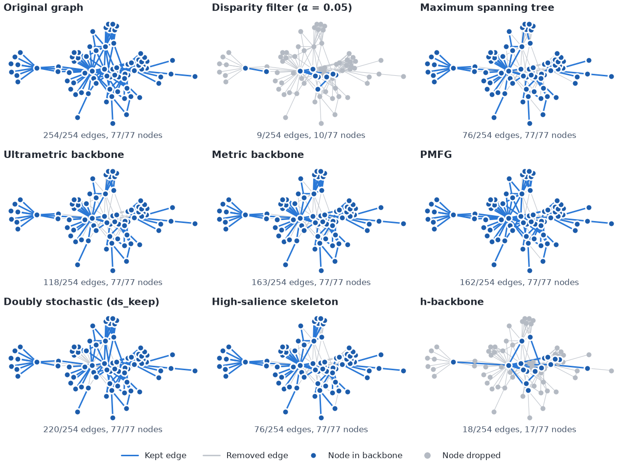
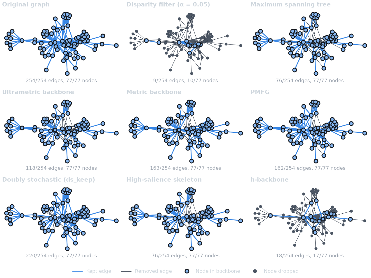
The picture shows sizes; the guarantees need checking. The table below tests each backbone, at build time, for four properties:

• Connected: every node of the network is still reachable from every other one (a backbone that drops a node fails this).

• Planar: it can be drawn without crossing edges.

• Shortest paths kept: the shortest-path distance between every pair of nodes, with distance 1/weight, is the same as in the full network.

• Minimax paths kept: the same for the minimax distance.

DISTANCE = "distance"


def with_distances(H):
    D = nx.Graph()
    D.add_nodes_from(G)
    D.add_edges_from((u, v, {DISTANCE: 1 / w}) for u, v, w in H.edges(data="weight"))
    return D


def shortest_paths(H):
    return dict(nx.all_pairs_dijkstra_path_length(with_distances(H), weight=DISTANCE))


def minimax_paths(H):
    # The minimax distance between two nodes is the longest step on the path
    # joining them in a minimum spanning forest of the distances.
    forest = nx.minimum_spanning_tree(with_distances(H), weight=DISTANCE)
    result = {}
    for source in forest:
        result[source] = {source: 0.0}
        for u, v in nx.bfs_edges(forest, source):
            result[source][v] = max(result[source][u], forest[u][v][DISTANCE])
    return result


def same_distances(full, part):
    return all(
        v in part[u] and math.isclose(d, part[u][v], rel_tol=1e-9)
        for u in full
        for v, d in full[u].items()
    )


full_sp, full_minimax = shortest_paths(G), minimax_paths(G)
checked = {
    **guarantee_backbones,
    "Disparity filter ∪ maximum spanning tree": nx.compose(
        guarantee_backbones["Disparity filter (α = 0.05)"],
        guarantee_backbones["Maximum spanning tree"],
    ),
}
rows = []
for name, backbone in checked.items():
    counts = style.backbone_counts(G, backbone)
    spanning = backbone.copy()
    spanning.add_nodes_from(G)
    rows.append(
        [
            name,
            counts.edges_kept,
            counts.nodes_kept,
            yes_no(nx.is_connected(spanning)),
            yes_no(nx.check_planarity(backbone)[0]),
            yes_no(same_distances(full_sp, shortest_paths(backbone))),
            yes_no(same_distances(full_minimax, minimax_paths(backbone))),
        ]
    )
Table(
    [
        "Backbone",
        "Edges",
        "Nodes",
        "Connected",
        "Planar",
        "Shortest paths kept",
        "Minimax paths kept",
    ],
    rows,
    caption=f"Properties checked on each backbone of the {G.number_of_edges()} edges.",
)

Properties checked on each backbone of the 254 edges.

Backbone	Edges	Nodes	Connected	Planar	Shortest paths kept	Minimax paths kept
Disparity filter (α = 0.05)	9	10	no	yes	no	no
Maximum spanning tree	76	77	yes	yes	no	yes
Ultrametric backbone	118	77	yes	no	no	yes
Metric backbone	163	77	yes	no	yes	yes
PMFG	162	77	yes	yes	no	yes
Doubly stochastic (ds_keep)	220	77	yes	no	no	no
High-salience skeleton	76	77	yes	yes	no	no
h-backbone	18	17	no	yes	no	no
Disparity filter ∪ maximum spanning tree	77	77	yes	yes	no	yes

Read the table as a menu of promises (the ultrametric backbone is also a subset of the metric one, which the next line checks).

ultra_edges = edge_set(guarantee_backbones["Ultrametric backbone"])
metric_edges = edge_set(guarantee_backbones["Metric backbone"])
print(f"ultrametric backbone inside the metric backbone: {ultra_edges <= metric_edges}")

ultrametric backbone inside the metric backbone: True

If you need a connected skeleton with as few edges as possible, the MST is the answer. If you will run shortest-path analyses (closeness, betweenness, routing) on the backbone, the metric backbone is the one that leaves them unchanged. The ultrametric backbone sits between the two: it contains every maximum spanning tree (section 3 shows why that matters). The PMFG keeps more structure than a tree, triangles in particular, while staying planar.

The disparity filter, by contrast, guarantees none of these. That is not a defect: it answers a different question, and its edges are the ones whose weights would be surprising under its null model. When you need both, a simple combination is the union of a significance backbone and an MST: it is connected and still contains every significant edge (the last row of the table).

2. Weights as strengths or as distances

The metric backbone, the ultrametric backbone and the salience all walk along paths, so they need a length for every edge. This library takes the weight as a strength (more co-appearances, a closer tie) and uses the distance 1/weight. That is right for counts, flows and similarities. It is wrong when the weight already is a length: a travel time, a physical distance, a dissimilarity.

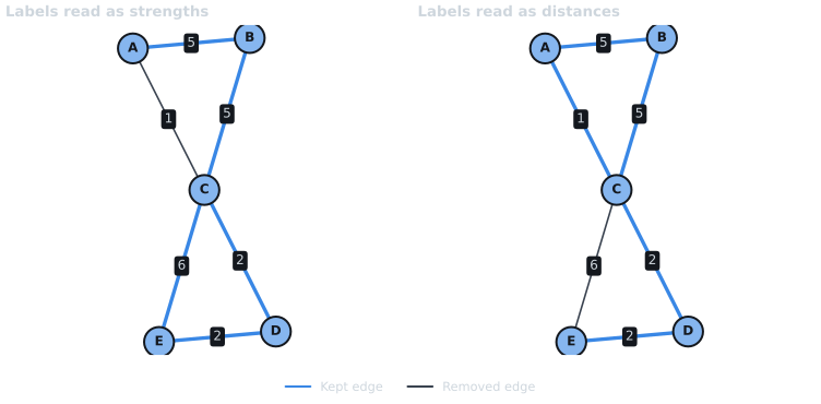
The same numbers can give opposite answers. In the small network below, read the labels first as strengths, then as distances. To make the library treat them as distances, pass their reciprocal as the weight.

toy = nx.Graph()
toy.add_weighted_edges_from(
    [
        ("A", "B", 5),
        ("B", "C", 5),
        ("A", "C", 1),
        ("C", "D", 2),
        ("D", "E", 2),
        ("C", "E", 6),
    ]
)
for *_, d in toy.edges(data=True):
    d["inverse"] = 1 / d["weight"]
toy_pos = style.layout(toy, "worked_example_paths", seed=7)
toy_views = {
    "Labels read as strengths": nb.boolean_filter(
        nb.metric_backbone(toy), "metric_keep"
    ),
    "Labels read as distances": nb.boolean_filter(
        nb.metric_backbone(toy, weight="inverse"), "metric_keep"
    ),
}


def removed_edges(backbone):
    return sorted("–".join(sorted(e)) for e in toy.edges() if not backbone.has_edge(*e))


def draw_toy(mode):
    p = style.palette(mode)
    fig, axes = plt.subplots(1, 2, figsize=(8, 3.8))
    for ax, (title, backbone) in zip(axes, toy_views.items()):
        style.draw_backbone(
            ax,
            toy,
            backbone,
            toy_pos,
            mode=mode,
            legend=False,
            title=title,
            node_size=420,
            kept_width=2.5,
            removed_width=1.2,
        )
        for u, v, w in toy.edges(data="weight"):
            (x1, y1), (x2, y2) = toy_pos[u], toy_pos[v]
            ax.text(
                (x1 + x2) / 2,
                (y1 + y2) / 2,
                f"{w:g}",
                ha="center",
                va="center",
                color=p.ink,
                zorder=5,
                bbox={"boxstyle": "round,pad=0.25", "fc": p.surface, "ec": "none"},
            )
        for node, (x, y) in toy_pos.items():
            ax.text(
                x,
                y,
                node,
                ha="center",
                va="center",
                color=p.surface,
                fontweight="bold",
                zorder=6,
            )
        ax.margins(0.18)
    fig.legend(
        handles=style.legend_handles(mode)[:2],
        loc="lower center",
        ncols=2,
        bbox_to_anchor=(0.5, -0.04),
    )
    fig.tight_layout(rect=(0, 0.05, 1, 1))
    return fig


Figure(
    draw_toy,
    "toy",
    alt=(
        "The same five-node network drawn twice, with the edge labels 5, 5, 1, "
        "2, 2 and 6. Left: the metric backbone when the labels are strengths. "
        "Right: the metric backbone when the labels are distances. Kept edges "
        "are thick and blue, the removed edge thin and gray."
    ),
    caption=(
        "Figure 2. One network, two readings of its weights. As strengths, the "
        f"metric backbone removes {', '.join(removed_edges(toy_views['Labels read as strengths']))}; "
        f"as distances, it removes {', '.join(removed_edges(toy_views['Labels read as distances']))}."
    ),
)

Figure 2. One network, two readings of its weights. As strengths, the metric backbone removes A–C; as distances, it removes C–E.

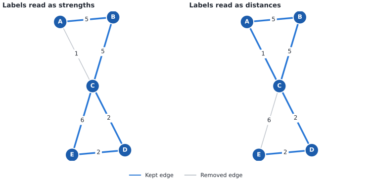
Read as strengths, A–C is a weak tie (distance 1) while the detour through B is two strong ties (distance 1/5 + 1/5), so A–C is redundant. Read as distances, A–C is the short hop and it stays; now the long edge C–E is the one with a shorter detour, through D. If your weights are lengths, invert them first, as above. transform_weights() records such a transform for describe_backbone(), and Weights, Units, and Transforms lists which methods care.

Salience follows the same convention. The salience of an edge is the share of nodes whose shortest-path tree (the union of the shortest paths from that node to all others) uses the edge. Here is the salience of every edge of the small network under both readings:

toy_salience = {
    reading: nb.high_salience_skeleton(toy, weight=attr)
    for reading, attr in (("strengths", "weight"), ("distances", "inverse"))
}
Table(
    ["Edge", "Label", "Salience, as strengths", "Salience, as distances"],
    [
        [
            f"{u}–{v}",
            f"{w:g}",
            f"{toy_salience['strengths'][u][v]['salience']:.2f}",
            f"{toy_salience['distances'][u][v]['salience']:.2f}",
        ]
        for u, v, w in toy.edges(data="weight")
    ],
    caption="Salience of each edge of the small network.",
)

Salience of each edge of the small network.

Edge	Label	Salience, as strengths	Salience, as distances
A–B	5	1.00	0.40
A–C	1	0.00	0.80
B–C	5	1.00	0.80
C–D	2	0.80	1.00
C–E	6	0.80	0.00
D–E	2	0.40	1.00

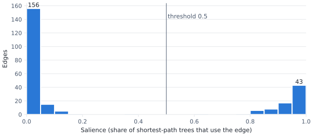
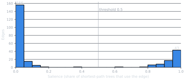
On Les Misérables salience is rarely in between: most edges are on almost every shortest-path tree or on almost none. That is why the threshold of 0.5 used in section 1 is not a delicate choice. Check the shape of the distribution on your own network before relying on it.

salience = [s for *_, s in nb.high_salience_skeleton(G).edges(data="salience")]
low = sum(s < 0.1 for s in salience)
high = sum(s > 0.9 for s in salience)
print(
    f"salience below 0.1: {low} edges; above 0.9: {high}; "
    f"in between: {len(salience) - low - high}"
)


def draw_salience(mode):
    p = style.palette(mode)
    fig, ax = plt.subplots(figsize=(7.5, 3))
    counts, edges, _ = ax.hist(
        salience,
        bins=np.linspace(0, 1, 21),
        color=p.kept,
        edgecolor=p.surface,
        linewidth=1.5,
    )
    ax.axvline(0.5, color=p.muted, linewidth=0.75)
    ax.text(0.505, counts.max() * 0.95, "threshold 0.5", color=p.muted, va="top")
    for i in (0, len(counts) - 1):
        ax.text(
            (edges[i] + edges[i + 1]) / 2,
            counts[i],
            f"{int(counts[i])}",
            ha="center",
            va="bottom",
            color=p.ink,
        )
    ax.set_xlabel("Salience (share of shortest-path trees that use the edge)")
    ax.set_ylabel("Edges")
    ax.set_xlim(0, 1)
    ax.grid(axis="y")
    return fig


Figure(
    draw_salience,
    "salience",
    alt=(
        "Histogram of edge salience in Les Misérables, in bins of 0.05 from 0 "
        "to 1. Almost all edges fall in the lowest or the highest bins, with "
        "very few in between; a vertical line marks the 0.5 threshold."
    ),
    caption=(
        f"Figure 3. Salience is bimodal: {low} edges have salience below 0.1 "
        f"and {high} above 0.9, out of {len(salience)}."
    ),
)

salience below 0.1: 171 edges; above 0.9: 60; in between: 23

Figure 3. Salience is bimodal: 171 edges have salience below 0.1 and 60 above 0.9, out of 254.

3. Ties and order dependence

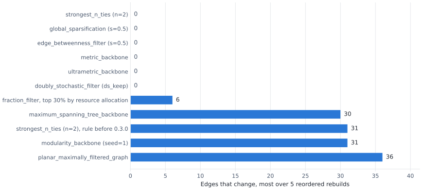
A method is order-dependent if building the same graph with its nodes and edges added in a different order can change the backbone. The cause is almost always a tie: two edges with equal weight (or equal score) where the method can only take one. Integer weights, like the counts here, tie often.

Version 0.3.0 removed this dependence from several methods (issues #60 and #64 on GitHub):

• strongest_n_ties() used to break ties at each node’s cutoff by adjacency order. Now a node selects every edge tied with its n-th strongest, so it can select more than n; this is the rule lspar() and local_degree() use.

• global_sparsification() and edge_betweenness_filter() break ties by the string form of the endpoints, now taken in sorted order, so the result no longer depends on how an edge was stored (it can still depend on the node labels).

Others still depend on order, for reasons their definitions make hard to avoid: the PMFG adds edges one at a time and takes tied edges in edge order; a maximum spanning tree is not unique when weights tie; the modularity backbone (Rajeh et al., 2022) runs Louvain community detection, whose visiting order follows node order even with a fixed seed; and fraction_filter() keeps an exact number of edges, so it breaks ties at its cut by input order, as its documentation says.

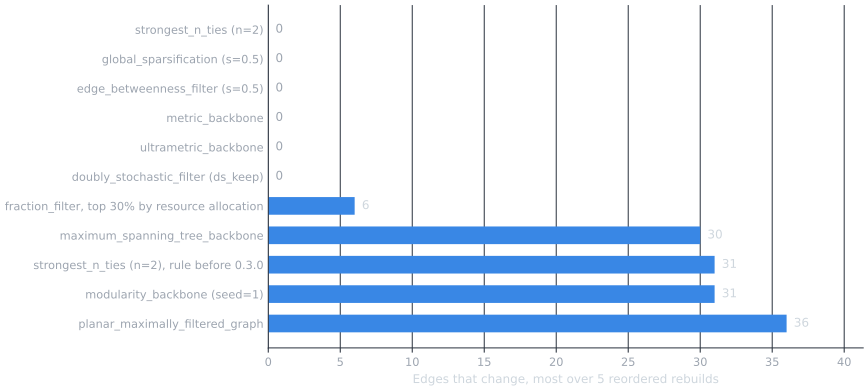
We measure this directly. Each method runs on the original graph and on five rebuilds with shuffled nodes and edges (and edges stored in random orientation); the chart counts the edges that change. For comparison, the first row re-implements the pre-0.3.0 strongest_n_ties rule.

def rebuild(H, seed):
    rng = random.Random(seed)
    nodes, edges = list(H.nodes(data=True)), list(H.edges(data=True))
    rng.shuffle(nodes)
    rng.shuffle(edges)
    R = H.__class__()
    R.add_nodes_from(nodes)
    for u, v, d in edges:
        R.add_edge(*((v, u) if rng.random() < 0.5 else (u, v)), **d)
    return R


def strongest_n_ties_before_0_3(H, n=2):
    """The old rule: per node, the n heaviest edges, ties by adjacency order."""
    kept = set()
    for u in H:
        nbrs = [(d.get("weight", 0), v) for v, d in H[u].items()]
        kept |= {
            frozenset((u, v)) for _, v in heapq.nlargest(n, nbrs, key=lambda x: x[0])
        }
    return kept


def unweighted(H):
    return nx.Graph(H.edges())


order_cases = {
    "strongest_n_ties (n=2), rule before 0.3.0": strongest_n_ties_before_0_3,
    "strongest_n_ties (n=2)": lambda H: edge_set(
        nb.boolean_filter(nb.strongest_n_ties(H, n=2), "strongest_n_ties_keep")
    ),
    "global_sparsification (s=0.5)": lambda H: edge_set(
        nb.boolean_filter(
            nb.global_sparsification(H, s=0.5), "global_sparsification_keep"
        )
    ),
    "edge_betweenness_filter (s=0.5)": lambda H: edge_set(
        nb.boolean_filter(nb.edge_betweenness_filter(H, s=0.5), "edge_betweenness_keep")
    ),
    "metric_backbone": lambda H: edge_set(
        nb.boolean_filter(nb.metric_backbone(H), "metric_keep")
    ),
    "ultrametric_backbone": lambda H: edge_set(
        nb.boolean_filter(nb.ultrametric_backbone(H), "ultrametric_keep")
    ),
    "doubly_stochastic_filter (ds_keep)": lambda H: edge_set(
        nb.boolean_filter(nb.doubly_stochastic_filter(H, smoothing=1e-4), "ds_keep")
    ),
    "planar_maximally_filtered_graph": lambda H: edge_set(
        nb.boolean_filter(nb.planar_maximally_filtered_graph(H), "pmfg_keep")
    ),
    "maximum_spanning_tree_backbone": lambda H: edge_set(
        nb.boolean_filter(nb.maximum_spanning_tree_backbone(H), "mst_keep")
    ),
    "modularity_backbone (seed=1)": lambda H: edge_set(
        nb.boolean_filter(nb.modularity_backbone(H, seed=1), "modularity_keep")
    ),
    "fraction_filter, top 30% by resource allocation": lambda H: edge_set(
        nb.fraction_filter(
            nb.resource_allocation_index(unweighted(H)),
            "resource_allocation",
            0.3,
            ascending=False,
        )
    ),
}
SEEDS = range(5)
rebuilds = [rebuild(G, seed) for seed in SEEDS]
order_rows = []
for name, method in order_cases.items():
    base = method(G)
    changed = [len(base ^ method(R)) for R in rebuilds]
    order_rows.append((name, len(base), changed))
order_rows.sort(key=lambda r: (max(r[2]) > 0, max(r[2])))


def draw_order(mode):
    p = style.palette(mode)
    fig, ax = plt.subplots(figsize=(8, 0.34 * len(order_rows) + 0.9))
    y = np.arange(len(order_rows))
    worst = [max(r[2]) for r in order_rows]
    ax.barh(y, worst, height=0.6, color=p.kept)
    for yi, value in zip(y, worst):
        ax.text(
            value + 0.5, yi, str(value), va="center", color=p.ink if value else p.muted
        )
    ax.set_yticks(y, [r[0] for r in order_rows])
    ax.invert_yaxis()
    ax.set_xlabel(f"Edges that change, most over {len(SEEDS)} reordered rebuilds")
    ax.set_xlim(0, max(worst) * 1.12 + 1)
    ax.grid(axis="x")
    ax.tick_params(axis="y", length=0)
    return fig


n_dependent = sum(max(r[2]) > 0 for r in order_rows)
Figure(
    draw_order,
    "order",
    alt=(
        "Horizontal bar chart, one bar per method, of how many backbone edges "
        "change when Les Misérables is rebuilt in a shuffled order. Methods "
        "with no change are listed first with the value 0; the order-dependent "
        "methods follow with longer bars. Every bar is labeled with its value."
    ),
    caption=(
        f"Figure 4. Order dependence on Les Misérables: {n_dependent} of "
        f"{len(order_rows)} rows change when the graph is rebuilt in another order."
    ),
)

Figure 4. Order dependence on Les Misérables: 5 of 11 rows change when the graph is rebuilt in another order.

The same numbers, for each rebuild:

Table(
    ["Method", "Edges on the original", "Edges changed in each rebuild"],
    [[name, size, ", ".join(map(str, changed))] for name, size, changed in order_rows],
    caption="Symmetric difference between the backbone of G and of each rebuild.",
)

Symmetric difference between the backbone of G and of each rebuild.

Method	Edges on the original	Edges changed in each rebuild
strongest_n_ties (n=2)	146	0, 0, 0, 0, 0
global_sparsification (s=0.5)	127	0, 0, 0, 0, 0
edge_betweenness_filter (s=0.5)	127	0, 0, 0, 0, 0
metric_backbone	163	0, 0, 0, 0, 0
ultrametric_backbone	118	0, 0, 0, 0, 0
doubly_stochastic_filter (ds_keep)	220	0, 0, 0, 0, 0
fraction_filter, top 30% by resource allocation	76	6, 4, 4, 4, 6
maximum_spanning_tree_backbone	76	28, 24, 30, 28, 20
strongest_n_ties (n=2), rule before 0.3.0	113	28, 31, 25, 30, 22
modularity_backbone (seed=1)	72	31, 26, 2, 9, 7
planar_maximally_filtered_graph	162	30, 36, 33, 35, 29

What to do about it:

• Need a tree-like, connected backbone? Prefer the ultrametric backbone to a single maximum spanning tree. An edge belongs to some maximum spanning tree exactly when no route between its endpoints has a shorter longest step, which is the ultrametric backbone’s rule, so it is the union of all maximum spanning trees and does not depend on order. The check below confirms that every tree the rebuilds produced lies inside it.

• Need a fixed number of edges? fraction_filter must break ties somewhere. If ties at the cut matter, use threshold_filter() at the score of the last kept edge instead: it keeps all tied edges, so it may keep a few more.

• PMFG and the modularity backbone: report the order you used, or run a few shuffles and keep the edges they agree on with consensus_backbone().

ultrametric = edge_set(guarantee_backbones["Ultrametric backbone"])
trees = [order_cases["maximum_spanning_tree_backbone"](R) for R in [G, *rebuilds]]
print(
    f"every maximum spanning tree found lies in the ultrametric backbone: "
    f"{all(tree <= ultrametric for tree in trees)}"
)
print(
    f"distinct trees found: {len({frozenset(t) for t in trees})} of {len(trees)}; "
    f"their union has {len(set().union(*trees))} edges, "
    f"the ultrametric backbone {len(ultrametric)}"
)

every maximum spanning tree found lies in the ultrametric backbone: True
distinct trees found: 6 of 6; their union has 109 edges, the ultrametric backbone 118

The resource-allocation row changes because of a tie exactly at the cut:

ra = nb.resource_allocation_index(U)
cut = 0.3
top = nb.fraction_filter(ra, "resource_allocation", cut, ascending=False)
cutoff = min(s for *_, s in top.edges(data="resource_allocation"))
tied = [e for e in ra.edges() if ra.edges[e]["resource_allocation"] == cutoff]
tied_kept = sum(top.has_edge(*e) for e in tied)
inclusive = nb.threshold_filter(
    ra, "resource_allocation", cutoff, mode="above", include_all_nodes=False
)
print(
    f"fraction_filter keeps {top.number_of_edges()} edges; {len(tied)} edges tie at "
    f"its cut score {cutoff:.4f} and {tied_kept} of them made it, by input order"
)
print(
    f"threshold_filter at that score keeps all of them: "
    f"{inclusive.number_of_edges()} edges"
)

fraction_filter keeps 76 edges; 15 edges tie at its cut score 0.7492 and 12 of them made it, by input order
threshold_filter at that score keeps all of them: 79 edges

4. Proximity scores for unweighted graphs

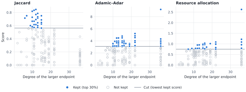
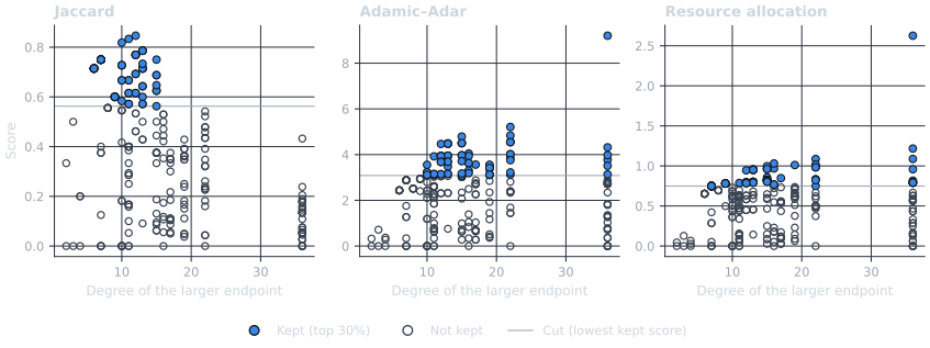
Without weights there is nothing to test against a null model of weights, but there is still structure. An edge whose endpoints share many neighbors is embedded in a dense group; an edge whose endpoints share none is a bridge between groups. A proximity score measures this overlap. Writing \(N(u)\) for the neighbors of u and \(k_z\) for the degree of a node z:

• Jaccard (Jaccard, 1901): \(|N(u) \cap N(v)| \,/\, |N(u) \cup N(v)|\), the share of the two neighborhoods that is common. A hub has a large union, so its edges score low.

• Adamic–Adar (Adamic & Adar, 2003): each common neighbor z counts \(1/\log k_z\). Sharing a well-connected neighbor counts for less.

• Resource allocation (Zhou et al., 2009): each common neighbor counts \(1/k_z\), a stronger discount for hubs as common neighbors, but no penalty for being a hub yourself.

Keeping the top 30% of edges by each score with fraction_filter() gives three backbones of equal size. Plotting each edge’s score against the degree of its better-connected endpoint shows what each one rewards.

proximity = {
    "Jaccard": ("jaccard", nb.jaccard_backbone(U)),
    "Adamic–Adar": ("adamic_adar", nb.adamic_adar_index(U)),
    "Resource allocation": ("resource_allocation", nb.resource_allocation_index(U)),
}
proximity_backbones = {
    name: nb.fraction_filter(H, attr, cut, ascending=False)
    for name, (attr, H) in proximity.items()
}
degree = dict(U.degree())
hub = max(degree, key=degree.get)


def draw_proximity_scatter(mode):
    p = style.palette(mode)
    fig, axes = plt.subplots(1, 3, figsize=(9, 3.3))
    for ax, (name, (attr, H)) in zip(axes, proximity.items()):
        backbone = proximity_backbones[name]
        kept = [backbone.has_edge(u, v) for u, v in H.edges()]
        x = np.array([max(degree[u], degree[v]) for u, v in H.edges()])
        y = np.array([s for *_, s in H.edges(data=attr)])
        k = np.array(kept)
        ax.scatter(
            x[~k],
            y[~k],
            s=22,
            facecolors="none",
            edgecolors=p.removed,
            linewidths=0.9,
            zorder=2,
        )
        ax.scatter(
            x[k], y[k], s=26, c=p.kept, edgecolors=p.surface, linewidths=0.8, zorder=3
        )
        ax.axhline(y[k].min(), color=p.muted, linewidth=0.75, zorder=1)
        ax.set_title(name)
        ax.set_xlabel("Degree of the larger endpoint")
        ax.grid(True)
    axes[0].set_ylabel("Score")
    marker = {"marker": "o", "linestyle": ""}
    fig.legend(
        handles=[
            Line2D(
                [],
                [],
                markerfacecolor=p.kept,
                markeredgecolor=p.surface,
                label=f"Kept (top {cut:.0%})",
                **marker,
            ),
            Line2D(
                [],
                [],
                markerfacecolor="none",
                markeredgecolor=p.removed,
                label="Not kept",
                **marker,
            ),
            Line2D(
                [], [], color=p.muted, linewidth=0.75, label="Cut (lowest kept score)"
            ),
        ],
        loc="lower center",
        ncols=3,
        bbox_to_anchor=(0.5, -0.03),
    )
    fig.tight_layout(rect=(0, 0.07, 1, 1))
    return fig


Figure(
    draw_proximity_scatter,
    "proximity_scatter",
    alt=(
        "Three scatter plots, one per score (Jaccard, Adamic–Adar, resource "
        "allocation), with one point per edge of the unweighted Les Misérables "
        "graph: the degree of the edge's better-connected endpoint on the "
        "horizontal axis and the score on the vertical axis. Kept edges are "
        "filled blue dots above a horizontal cut line; the others are hollow "
        "gray circles. Jaccard keeps almost no edges at high degree; the other "
        "two keep many."
    ),
    caption=(
        f"Figure 5. What each score rewards. Each panel keeps the top {cut:.0%} "
        "of edges (filled dots, above the cut line)."
    ),
)

Figure 5. What each score rewards. Each panel keeps the top 30% of edges (filled dots, above the cut line).

The same three backbones on the network, with the best-connected character labeled:

def draw_proximity_backbones(mode):
    p = style.palette(mode)
    fig, axes = plt.subplots(1, 3, figsize=(9, 3.9))
    for ax, (name, backbone) in zip(axes, proximity_backbones.items()):
        counts = style.draw_backbone(
            ax, U, backbone, pos, mode=mode, legend=False, title=name
        )
        x, y = pos[hub]
        ax.annotate(
            hub,
            (x, y),
            xytext=(0, 9),
            textcoords="offset points",
            ha="center",
            color=p.ink,
            fontsize=8.5,
            bbox={"boxstyle": "round,pad=0.2", "fc": p.surface, "ec": "none"},
            zorder=6,
        )
        ax.text(
            0.5,
            -0.01,
            counts.short,
            transform=ax.transAxes,
            ha="center",
            va="top",
            color=p.muted,
            fontsize=8.5,
        )
    fig.legend(
        handles=style.legend_handles(mode),
        loc="lower center",
        ncols=4,
        bbox_to_anchor=(0.5, -0.03),
    )
    fig.tight_layout(rect=(0, 0.08, 1, 1))
    return fig


hub_edges = {
    name: sum(hub in e for e in backbone.edges())
    for name, backbone in proximity_backbones.items()
}
Figure(
    draw_proximity_backbones,
    "proximity_backbones",
    fmt="png",
    alt=(
        "Three network drawings of the unweighted Les Misérables graph on the "
        f"shared layout, with the hub {hub} labeled: the top {cut:.0%} of edges "
        "by Jaccard, by Adamic–Adar and by resource allocation. Kept edges are "
        "thick and blue, removed edges thin and gray."
    ),
    caption=(
        f"Figure 6. Three proximity backbones of equal size. {hub} has "
        f"{degree[hub]} edges and keeps "
        + ", ".join(f"{k} under {name}" for name, k in hub_edges.items())
        + "."
    ),
)

Figure 6. Three proximity backbones of equal size. Valjean has 36 edges and keeps 0 under Jaccard, 6 under Adamic–Adar, 10 under Resource allocation.

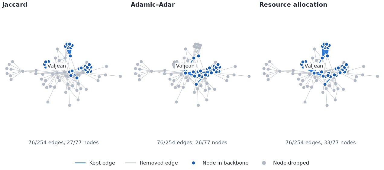
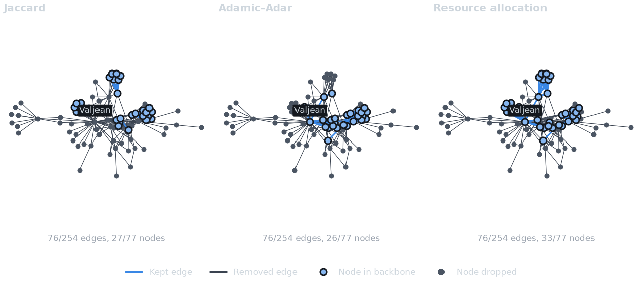
Jaccard favors tight groups of characters with similar circles and drops the hub’s edges; the two common-neighbor indices keep them, since the hub shares many neighbors with the characters around it. Pick Jaccard to reveal communities, a common-neighbor index to keep the core. The three scores agree on part of the backbone:

names = list(proximity_backbones)
Table(
    ["Pair of scores", "Edges in both", "Edges in either"],
    [
        [
            f"{a} and {b}",
            len(edge_set(proximity_backbones[a]) & edge_set(proximity_backbones[b])),
            len(edge_set(proximity_backbones[a]) | edge_set(proximity_backbones[b])),
        ]
        for i, a in enumerate(names)
        for b in names[i + 1 :]
    ],
    caption=f"Overlap of the three top-{cut:.0%} backbones.",
)

Overlap of the three top-30% backbones.

Pair of scores	Edges in both	Edges in either
Jaccard and Adamic–Adar	41	111
Jaccard and Resource allocation	44	108
Adamic–Adar and Resource allocation	46	106

Sparsifiers: a budget per node

A global cut such as the top 30% can strip small or peripheral nodes of every edge. A sparsifier instead gives every node a budget that grows with its degree d: each node keeps its best ceil(d**s) edges, and an edge stays if either endpoint keeps it. The exponent s runs from 0 (one edge per node) to 1 (everything).

• lspar() (Satuluri et al., 2011) ranks each node’s edges by Jaccard similarity.

• local_degree() (Lindner et al., 2015) ranks a node’s edges by the degree of the neighbor and keeps floor(d**s) (at least one), so every node stays attached toward the hubs.

• sparsify() is the general pipeline that both follow (Neal, 2022). With umst=True it also adds the union of all minimum spanning trees of the edges’ scores (Hamann et al., 2016), so the backbone keeps the network’s connected components.

• lspar(convention="r") reproduces R backbone’s backbone_from_unweighted(model = "lspar"). R ignores edges in no triangle, divides by a smaller union and keeps floor(d**s) edges with no minimum, so it keeps fewer edges and can drop nodes. Use it to match results computed in R, not as a default.

All four run at the same exponent here.

s = 0.3
sparsifiers = {
    f"lspar (s={s})": nb.lspar(U, s=s),
    f'lspar (s={s}, convention="r")': nb.lspar(U, s=s, convention="r"),
    f"local_degree (s={s})": nb.local_degree(U, s=s),
    f"sparsify (s={s}, umst=True)": nb.sparsify(U, s=s, umst=True),
}
sparse_backbones = {
    name: nb.boolean_filter(H, "sparsify_keep") for name, H in sparsifiers.items()
}


def components(backbone):
    kept = nx.Graph(backbone.edges())
    return nx.number_connected_components(kept) if len(kept) else 0


def draw_sparsifiers(mode):
    p = style.palette(mode)
    fig, axes = plt.subplots(2, 2, figsize=(8, 5.6))
    for ax, (name, backbone) in zip(axes.flat, sparse_backbones.items()):
        counts = style.draw_backbone(
            ax, U, backbone, pos, mode=mode, legend=False, title=name
        )
        ax.text(
            0.5,
            -0.01,
            f"{counts.short}, {components(backbone)} component(s)",
            transform=ax.transAxes,
            ha="center",
            va="top",
            color=p.muted,
            fontsize=8.5,
        )
    fig.legend(
        handles=style.legend_handles(mode),
        loc="lower center",
        ncols=4,
        bbox_to_anchor=(0.5, -0.01),
    )
    fig.tight_layout(rect=(0, 0.04, 1, 1))
    return fig


Figure(
    draw_sparsifiers,
    "sparsifiers",
    fmt="png",
    alt=(
        "Four network drawings of the unweighted Les Misérables graph on the "
        f"shared layout: lspar, lspar with R's convention, local degree, and "
        f"sparsify with the union of minimum spanning trees, all at s = {s}. "
        "Each panel lists its kept edges, kept nodes and connected components."
    ),
    caption=(
        f"Figure 7. Four sparsifiers at s = {s}. "
        + " ".join(
            f"{name}: {style.backbone_counts(U, b).edges_kept} edges, "
            f"{components(b)} component(s)."
            for name, b in sparse_backbones.items()
        )
    ),
)

Figure 7. Four sparsifiers at s = 0.3. lspar (s=0.3): 154 edges, 3 component(s). lspar (s=0.3, convention="r"): 101 edges, 10 component(s). local_degree (s=0.3): 91 edges, 1 component(s). sparsify (s=0.3, umst=True): 156 edges, 1 component(s).

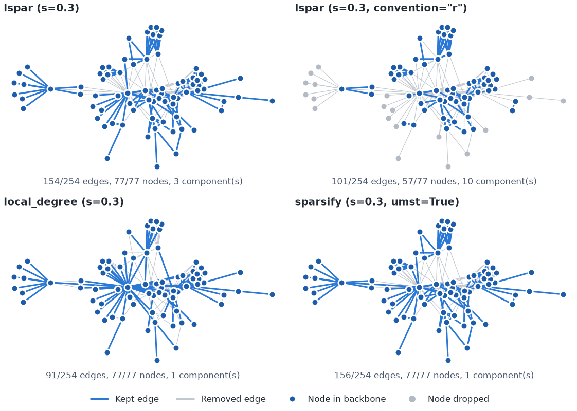
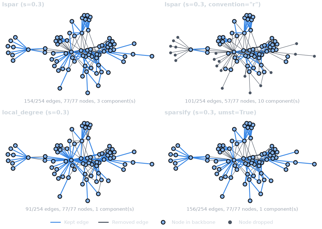
Local degree keeps every character attached, by its edge to the best-connected neighbor, and umst=True turns lspar’s pieces back into one network at the cost of a few edges. Because every one of these methods keeps edges tied at a node’s cutoff together, none of them depends on input order.

5. The doubly stochastic filter

Weights are hard to compare across nodes of very different strength: a weight of 5 is most of a minor character’s ties and a small part of the hero’s. The doubly stochastic filter (Slater, 2009) removes that difference. It rescales the weight matrix until every row and every column sums to one, a doubly stochastic matrix, by the Sinkhorn–Knopp iteration: divide each row by its sum, then each column by its sum, and repeat. The rescaled weight is stored as ds_weight. A second stage then adds edges from the largest ds_weight down until the network is connected and flags them ds_keep.

The iteration converges only if the matrix has total support, which sparse networks often lack. Two leaves (nodes of degree one) hanging off the same node are enough to prevent it: a leaf’s row has a single nonzero entry, which would have to be 1, and two such entries in the shared neighbor’s column already sum to 2. Les Misérables has several such nodes:

leaves = {n for n in G if G.degree(n) == 1}
crowded = sorted(n for n in G if sum(nbr in leaves for nbr in G[n]) >= 2)
print(f"nodes with two or more leaves attached: {', '.join(crowded)}")

nodes with two or more leaves attached: Myriel, Valjean

smoothing= adds a small pseudocount to every cell of the matrix, edges and non-edges alike, which makes every matrix scalable. It changes the scores slightly, since part of each node’s unit sum now goes to non-edges, so keep it small relative to the weights; netbone uses 1e-4.

To see the convergence, the code below repeats the library’s iteration and records the largest deviation of a row or column sum from one after each step. It checks that it ends on the library’s own ds_weight.

MAX_ITER, TOL = 1000, 1e-8
nodes = list(G)
A = nx.to_numpy_array(G, nodelist=nodes, weight="weight")


def sinkhorn_trace(smoothing):
    M = A + smoothing * (1 - np.eye(len(A)))
    active = M.sum(axis=1) > 0
    D, trace = M.copy(), []
    for _ in range(MAX_ITER):
        D = D / D.sum(axis=1, keepdims=True)
        D = D / D.sum(axis=0, keepdims=True)
        rs, cs = D.sum(axis=1)[active], D.sum(axis=0)[active]
        trace.append(max(np.abs(rs - 1).max(), np.abs(cs - 1).max()))
        if np.allclose(rs, 1, rtol=0, atol=TOL) and np.allclose(
            cs, 1, rtol=0, atol=TOL
        ):
            break
    return trace, np.sqrt(D * D.T)


ds_runs = {}
for smoothing in (0.0, 1e-6, 1e-4):
    with warnings.catch_warnings(record=True) as caught:
        warnings.simplefilter("always")
        H = nb.doubly_stochastic_filter(
            G, smoothing=smoothing, max_iter=MAX_ITER, tol=TOL
        )
    trace, D = sinkhorn_trace(smoothing)
    idx = {n: i for i, n in enumerate(nodes)}
    assert all(
        math.isclose(d, D[idx[u], idx[v]], rel_tol=1e-9, abs_tol=1e-300)
        for u, v, d in H.edges(data="ds_weight")
    )
    ds_runs[smoothing] = {"trace": trace, "warned": bool(caught), "scored": H}


def draw_convergence(mode):
    p = style.palette(mode)
    colors = style.categorical(len(ds_runs), mode)
    fig, ax = plt.subplots(figsize=(7.5, 3.6))
    for color, (smoothing, run) in zip(colors, ds_runs.items()):
        it = np.arange(1, len(run["trace"]) + 1)
        label = f"smoothing = {smoothing:g}"
        ax.plot(it, run["trace"], color=color, label=label)
        ax.annotate(
            label,
            (it[-1], run["trace"][-1]),
            xytext=(5, 4),
            textcoords="offset points",
            va="bottom",
            color=p.ink,
        )
    ax.axhline(TOL, color=p.muted, linewidth=0.75)
    ax.text(MAX_ITER * 1.24, TOL, f"tol = {TOL:g}", color=p.muted, ha="right", va="top")
    ax.set_yscale("log")
    ax.set_xlim(0, MAX_ITER * 1.25)
    ax.set_ylim(TOL / 10, None)
    ax.set_xlabel("Sinkhorn–Knopp iteration")
    ax.set_ylabel("Largest |row or column sum − 1|")
    ax.grid(True)
    fig.legend(loc="lower center", ncols=len(ds_runs), bbox_to_anchor=(0.5, -0.03))
    fig.tight_layout(rect=(0, 0.07, 1, 1))
    return fig


Figure(
    draw_convergence,
    "convergence",
    alt=(
        "Line chart on a logarithmic vertical axis: the largest deviation of a "
        "row or column sum from one, against the Sinkhorn–Knopp iteration, for "
        "three smoothing values. Each line is labeled at its end. A horizontal "
        "line marks the tolerance; only lines that reach it converged."
    ),
    caption=(
        "Figure 8. Convergence of Sinkhorn–Knopp on Les Misérables. "
        + " ".join(
            f"smoothing={sm:g}: "
            + (
                f"stops after {len(r['trace'])} iterations."
                if not r["warned"]
                else f"no convergence in {MAX_ITER} iterations."
            )
            for sm, r in ds_runs.items()
        )
    ),
)

Figure 8. Convergence of Sinkhorn–Knopp on Les Misérables. smoothing=0: no convergence in 1000 iterations. smoothing=1e-06: no convergence in 1000 iterations. smoothing=0.0001: stops after 290 iterations.

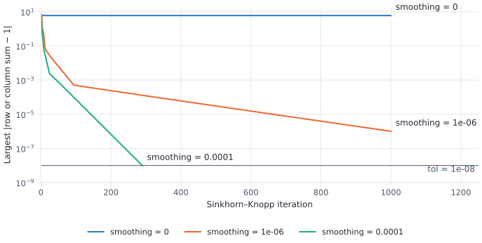
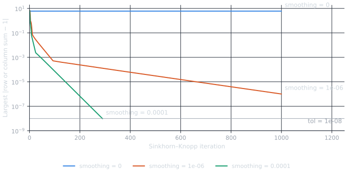
Without smoothing the deviation stalls far above the tolerance and the function warns. ds_weight then holds the last iterate, whose entries for the unsupported edges shrink toward zero, some all the way to exactly 0. An edge of weight 0 cannot join two components, so the second stage can no longer connect the network, as the function’s Notes explain. A pseudocount repairs this; the smaller it is, the more iterations it needs (raise max_iter if the function still warns):

rows = []
for smoothing, run in ds_runs.items():
    H = run["scored"]
    backbone = nb.boolean_filter(H, "ds_keep")
    rows.append(
        [
            f"{smoothing:g}",
            yes_no(not run["warned"]),
            len(run["trace"]),
            sum(d == 0 for *_, d in H.edges(data="ds_weight")),
            backbone.number_of_edges(),
            yes_no(nx.is_connected(backbone)),
        ]
    )
Table(
    [
        "smoothing",
        "Converged",
        "Iterations",
        "ds_weight = 0",
        "ds_keep edges",
        "ds_keep connected",
    ],
    rows,
    caption=f"The doubly stochastic filter on Les Misérables (max_iter={MAX_ITER}).",
)

The doubly stochastic filter on Les Misérables (max_iter=1000).

smoothing	Converged	Iterations	ds_weight = 0	ds_keep edges	ds_keep connected
0	no	1000	53	187	no
1e-06	no	1000	0	220	yes
0.0001	yes	290	0	220	yes

Where next

• API reference: Structural Methods, Proximity Methods, Unweighted Sparsification and Filters.

• How-to tutorials with every method of each family: Structural Backbone Methods, Proximity-Based Edge Scoring, Unweighted Graph Sparsification.

• Choosing among families, and comparing the results: Choosing a Method, Comparing Multiple Methods, Validating a Backbone and Les Miserables Benchmark.

• Weights that are lengths, or need a transform first: Weights, Units, and Transforms.

References

The citations above are the library’s own: each is taken from nx_backbone.describe.REFERENCES, the bibliography that describe_backbone() uses, and checked against it here.

cited = {
    "tumminello2005": "Tumminello et al., 2005",
    "simas2021": "Simas et al., 2021",
    "slater2009": "Slater, 2009",
    "grady2012": "Grady et al., 2012",
    "zhang2018": "Zhang et al., 2018",
    "serrano2009": "Serrano et al., 2009",
    "rajeh2022": "Rajeh et al., 2022",
    "jaccard1901": "Jaccard, 1901",
    "adamic2003": "Adamic & Adar, 2003",
    "zhou2009": "Zhou et al., 2009",
    "satuluri2011": "Satuluri et al., 2011",
    "lindner2015": "Lindner et al., 2015",
    "neal2022": "Neal, 2022",
    "hamann2016": "Hamann et al., 2016",
}
assert all(REFERENCES[key].cite() == text for key, text in cited.items())
methods_used = [
    "planar_maximally_filtered_graph",
    "metric_backbone",
    "ultrametric_backbone",
    "doubly_stochastic_filter",
    "high_salience_skeleton",
    "h_backbone",
    "disparity_filter",
    "modularity_backbone",
    "jaccard_backbone",
    "adamic_adar_index",
    "resource_allocation_index",
    "lspar",
    "local_degree",
    "sparsify",
]
assert {k for m in methods_used for k in METHODS[m].refs} <= set(cited)


class ReferenceList:
    """The full references, as an HTML list."""

    def __init__(self, keys):
        self.keys = keys

    def _repr_html_(self):
        items = "".join(
            f"<li>{html.escape(REFERENCES[k].text())}</li>" for k in self.keys
        )
        return f"<ul>{items}</ul>"


ReferenceList(sorted(cited))

• Adamic, L. A., & Adar, E. (2003). Friends and neighbors on the Web. Social Networks, 25(3), 211-230.
• Grady, D., Thiemann, C., & Brockmann, D. (2012). Robust classification of salient links in complex networks. Nature Communications, 3, 864. https://doi.org/10.1038/ncomms1847
• Hamann, M., Lindner, G., Meyerhenke, H., Staudt, C. L., & Wagner, D. (2016). Structure-preserving sparsification methods for social networks. Social Network Analysis and Mining, 6(1), 22. https://doi.org/10.1007/s13278-016-0332-2
• Jaccard, P. (1901). Distribution de la flore alpine dans le bassin des Dranses et dans quelques regions voisines. Bulletin de la Societe Vaudoise des Sciences Naturelles, 37, 241-272.
• Lindner, G., Staudt, C. L., Hamann, M., Meyerhenke, H., & Wagner, D. (2015). Structure-preserving sparsification of social networks. Proceedings of the 2015 IEEE/ACM International Conference on Advances in Social Networks Analysis and Mining (ASONAM), 448-454.
• Neal, Z. P. (2022). backbone: An R package to extract network backbones. PLoS ONE, 17(5), e0269137. https://doi.org/10.1371/journal.pone.0269137
• Rajeh, S., Savonnet, M., Leclercq, E., & Cherifi, H. (2022). Modularity-based backbone extraction in weighted complex networks. NetSci-X 2022, 67-79.
• Satuluri, V., Parthasarathy, S., & Ruan, Y. (2011). Local graph sparsification for scalable clustering. Proceedings of the ACM SIGMOD International Conference on Management of Data, 721-732. https://doi.org/10.1145/1989323.1989399
• Serrano, M. A., Boguñá, M., & Vespignani, A. (2009). Extracting the multiscale backbone of complex weighted networks. Proceedings of the National Academy of Sciences, 106(16), 6483-6488. https://doi.org/10.1073/pnas.0808904106
• Simas, T., Correia, R. B., & Rocha, L. M. (2021). The distance backbone of complex networks. Journal of Complex Networks, 9(6), cnab021. https://doi.org/10.1093/comnet/cnab021
• Slater, P. B. (2009). A two-stage algorithm for extracting the multiscale backbone of complex weighted networks. Proceedings of the National Academy of Sciences, 106(26), E66.
• Tumminello, M., Aste, T., Di Matteo, T., & Mantegna, R. N. (2005). A tool for filtering information in complex systems. Proceedings of the National Academy of Sciences, 102(30), 10421-10426.
• Zhang, R. J., Stanley, H. E., & Ye, F. Y. (2018). Extracting h-backbone as a core structure in weighted networks. Scientific Reports, 8, 14356.
• Zhou, T., Lü, L., & Zhang, Y.-C. (2009). Predicting missing links via local information. European Physical Journal B, 71(4), 623-630.