Temporal#
Temporal networks as snapshots, timestamped events, or spans, conversions between the three forms, and temporal backbone scores and tests. The Temporal networks: formats and conversions guide walks through every conversion with examples and a table of what each one keeps; the Temporal Backbones tutorial compares the scores on synthetic snapshots, and Temporal backbones: presence and eligible steps explains how absent edges are counted. The narrative tutorial Temporal backbones, from snapshots to smoothing follows one case from raw records to a backbone, with figures, and compares the methods.
Temporal networks: input forms and conversions between them.
NetworkX has no temporal graph class, so nx_backbone.temporal
accepts a network observed over time in any of three forms, all built from
ordinary NetworkX graphs:
Snapshots: a dict
{t: G_t}ofGraphorDiGraphobjects whose keys are mutually comparable times, or a list[G_0, ..., G_{T-1}], read as times0, ..., T - 1. All snapshots are directed or all are undirected; multigraph snapshots are rejected. A node is present at timetif it is inG_t, isolated or not.Events: one
MultiGraphorMultiDiGraphwith one edge per event. Each edge carries its time in thetimeattribute, plus any other attributes such asweight.Spans: one
MultiGraphorMultiDiGraphwith one edge per contact that lasts. Each edge carriesstartandendattributes. A span covers the half-open interval[start, end): it includes its start and excludes its end, so a span that ends at 5 and one that starts at 5 touch without overlapping. A span withstart == endis an instantaneous contact atstart.
Every function takes the attribute names as keywords (time=, start=,
end=), and temporal_form() tells the three forms apart.
Binning. Events and spans become snapshots by binning time into steps of
width freq=, starting at origin= (default: the earliest time). Bin
k is the half-open interval [origin + k * freq, origin + (k + 1) *
freq) and its snapshot is keyed by its start. An event belongs to the bin
that contains its time; a span belongs to every bin it overlaps (its interval
and the bin’s intersect), so a span from 0 to 10 is observed in each of five
bins of width 2. Snapshots run from the first to the last occupied bin;
empty bins in between are kept as empty graphs. The parallel edges of a node
pair within one bin collapse into one edge with
multigraph_to_weighted() (aggregate="sum" by
default): its weight combines their weights (a missing weight counts as
1) and edge_count counts them. Attributes on which all of them agree are
kept. A node is present in a bin only if it has an event or span there.
Times. Plain numbers work with NetworkX alone, as do
datetime.datetime times with a datetime.timedelta step.
pandas is needed only for frequency strings such as freq="1D" (or pandas
offsets such as "MS", which step by calendar months) and for the
DataFrame functions from_event_table() and to_event_table();
it is imported lazily, only on those paths. pandas Timestamp and
Timedelta values work wherever datetimes do.
Round trips. Converting snapshots to events or spans loses what an edge
list cannot hold: empty snapshots, isolated nodes, and per-snapshot node and
graph attributes. events_from_snapshots() and
spans_from_snapshots() therefore store that information in the graph
attribute M.graph["temporal"], a dict with keys "form" ("events"
or "spans"), "times" (the snapshot times in order), "snapshots"
(for each time, the snapshot’s graph attributes, "graph", and its nodes
with their attributes, "nodes") and, for spans, "end_time" (when the
last snapshot ends). snapshots_from_events() and
snapshots_from_spans() called without freq and origin use this
record to return the original snapshots exactly (as a dict, up to the order
of edges): the same times, nodes, edges, and node, edge and graph attributes.
The record describes the snapshots as they were converted. If the events or
spans no longer fit it (a time that is not a recorded snapshot time, or two
edges of one node pair in one snapshot), it is ignored and the input is
binned as usual. The other directions aggregate and are lossy; each
function’s Notes say what is kept.
Temporal backbone scores. observation_fraction(),
persistence(),
backbone_stability() and
weight_trend() take any of the three forms (events
and spans are binned first, with freq=) and score every edge over the
resulting steps. An edge’s eligible steps are those in which both of its
endpoints are present. In an eligible step an absent edge is an observed
zero (weight 0); in any other step the edge is unknown and is not counted, so
an edge whose endpoint joins late is scored only from the step it joins.
Each scorer returns one static graph: the
flatten_temporal() of the steps (a
Graph, or DiGraph for directed input,
with every node of every step and its attributes from the latest step it is
in), restricted to the observed edges, which carry their score attributes.
H.graph["temporal"] records the method, the
input form, the step times, n_steps, freq, origin and the
parameters. The usual filters then apply, as in
threshold_filter(H, "obs_fraction", 0.5, mode="above"). The scores are
descriptive: they come without p-values. All but
weight_trend() work with NetworkX alone (numpy, when
installed, vectorizes them).
Model-based scores. edge_persistence_hmm()
(numpy) follows the same input and output conventions. It treats each edge
as a two-state hidden Markov chain (inactive or active) observed with error
in its eligible steps (the other steps carry no evidence), and adds
posterior activity scores plus a per-step hmm_posterior dict; the fitted
model is in H.graph["temporal"]["hmm"].
kalman_backbone() (numpy and SciPy) tests every edge
in every step with a static significance test and smooths each edge’s
evidence over time with a Kalman filter and smoother. It adds an edge-level
kalman_pvalue and per-step series as dict attributes keyed by time;
kalman_snapshots() expands those into one graph per
step, and the fitted model is in H.graph["temporal"]["kalman"].
Temporal backbone scores
Each takes any of the three forms (freq= and origin= bin events and
spans into steps) and returns one scored static graph, filtered with
threshold_filter() and the other filters. These
scores are descriptive: they come without p-values. They are not dispatchable to
NetworkX backends, because they take several graphs or a multigraph of events
rather than one graph.
- nx_backbone.observation_fraction(T, *, weight=None, min_weight=0, freq=None, origin=None, time='time', start='start', end='end', aggregate='sum')[source]#
Score each edge by the share of its eligible steps in which it is observed.
An edge’s eligible steps are those in which both of its endpoints are present. In an eligible step the edge is either observed or an observed zero; in the other steps it is unknown and not counted.
- Parameters:
- Tdict, list, MultiGraph or MultiDiGraph
A temporal network: snapshots (a dict
{time: graph}or a list of graphs), or a multigraph of events or spans (seenx_backbone.temporal).- weightstr or None, optional (default=None)
If given, an edge counts as observed only when its weight is above min_weight (a missing weight counts as 1).
Nonecounts every edge present in a step.- min_weightfloat, optional (default=0)
The weight an observed edge must exceed when weight is given.
- freqnumber, timedelta, str or None, optional (default=None)
Step width for binning events or spans into snapshots, as in
snapshots_from_events(): a number for numeric times, adatetime.timedeltaor a pandas frequency string such as"1D"(pandas only) for datetimes.Nonemakes one step per distinct time. Snapshots are already steps, so freq must beNonefor them.- origintime or None, optional (default=None)
Start of the first bin (default: the earliest time); with freq only.
- timestr, optional (default=”time”)
Edge attribute holding an event’s time.
- start, endstr, optional (default=”start”, “end”)
Edge attributes holding a span’s start and end.
- aggregate{“sum”, “count”, “max”, “min”, “mean”}, optional (default=”sum”)
How the weights of a node pair’s events or spans in one bin combine (see
multigraph_to_weighted()).
- Returns:
- HGraph or DiGraph
The union of the edges observed in any step, with the attributes
flatten_temporal()gives them over the steps (the summed weight,n_obs,first,last, and the attributes all their observations share), plusobs_fraction:n_obs / n_eligible;n_obs: the number of steps in which the edge is observed (replacing the count offlatten_temporal(), which also counts the steps where the weight is at most min_weight);n_eligible: the number of steps in which both endpoints are present;first_obs,last_obs: the times of the first and last observation.
Nodes are every node present in any step, with their attributes from the latest step they are in, and graph attributes come from the latest step.
H.graph["temporal"]records the method, the input form, the step times,n_steps, freq, origin and the parameters.
- Raises:
- NetworkXNotImplemented
If a snapshot is a multigraph.
- NetworkXError
If weight is given and a weight is not numeric, or T is not a temporal network.
- ValueError
If freq or origin is given with snapshots, or the input has no steps.
See also
persistenceTell steady edges from intermittent ones.
threshold_filterKeep the edges above a chosen fraction.
Notes
A node is present in a snapshot if it is in that graph, isolated or not; after binning events or spans, a node is present in a step only if it has an event or span there. So an edge whose endpoint joins late is scored only on the steps after it joins.
Examples
Node
"c"joins at time 3, so the edge("b", "c")has two eligible steps and is observed in both;("a", "b")is absent at time 4 while both endpoints are present, an observed zero:>>> import networkx as nx >>> import nx_backbone as nb >>> S = { ... 1: nx.Graph([("a", "b")]), ... 2: nx.Graph([("a", "b")]), ... 3: nx.Graph([("a", "b"), ("b", "c")]), ... 4: nx.Graph([("b", "c"), ("a", "z")]), ... } >>> H = nb.observation_fraction(S) >>> H["a"]["b"] {'weight': 3, 'n_obs': 3, 'first': 1, 'last': 3, 'obs_fraction': 0.75, 'n_eligible': 4, 'first_obs': 1, 'last_obs': 3} >>> H["b"]["c"]["obs_fraction"] 1.0 >>> B = nb.threshold_filter(H, "obs_fraction", 0.8, mode="above") >>> sorted(tuple(sorted(e)) for e in B.edges) [('a', 'z'), ('b', 'c')]
Computational complexity estimate is
O(n_S + m_S + m T)time andO(n T + m T)space.
- nx_backbone.persistence(T, *, weight=None, min_weight=0, ineligible='skip', freq=None, origin=None, time='time', start='start', end='end', aggregate='sum')[source]#
Score each edge by its runs of consecutive observed steps.
A run is a maximal sequence of consecutive eligible steps (both endpoints present) in which the edge is observed. An edge seen in steps 1-10 has one run of 10; an edge seen in 10 scattered steps has many short runs, although both have the same
observation_fraction().- Parameters:
- Tdict, list, MultiGraph or MultiDiGraph
A temporal network: snapshots (a dict
{time: graph}or a list of graphs), or a multigraph of events or spans (seenx_backbone.temporal).- weightstr or None, optional (default=None)
If given, an edge counts as observed only when its weight is above min_weight (a missing weight counts as 1).
- min_weightfloat, optional (default=0)
The weight an observed edge must exceed when weight is given.
- ineligible{“skip”, “break”}, optional (default=”skip”)
How steps in which an endpoint is absent (unknown for the edge) count.
"skip"passes over them: they neither break nor extend a run, and a step’s next step is the next eligible one."break"treats them as unobserved, so they end a run, and a step’s next step is simply the following step.- freqnumber, timedelta, str or None, optional (default=None)
Step width for binning events or spans into snapshots, as in
snapshots_from_events(): a number for numeric times, adatetime.timedeltaor a pandas frequency string such as"1D"(pandas only) for datetimes.Nonemakes one step per distinct time. Snapshots are already steps, so freq must beNonefor them.- origintime or None, optional (default=None)
Start of the first bin (default: the earliest time); with freq only.
- timestr, optional (default=”time”)
Edge attribute holding an event’s time.
- start, endstr, optional (default=”start”, “end”)
Edge attributes holding a span’s start and end.
- aggregate{“sum”, “count”, “max”, “min”, “mean”}, optional (default=”sum”)
How the weights of a node pair’s events or spans in one bin combine (see
multigraph_to_weighted()).
- Returns:
- HGraph or DiGraph
The union of the edges observed in any step, with the attributes
flatten_temporal()gives them over the steps (the summed weight,n_obs,first,last, and the attributes all their observations share), plusmax_run: the length of the longest run, in steps;mean_run: the mean run length;n_runs: the number of runs;persistence: the share of the edge’s observed steps whose next step is also observed, an empirical “stays active” probability. Observed steps without a next step (the edge’s last eligible step, or the last step) are left out;persistenceis NaN when no observed step has a next step.
Nodes and
H.graph["temporal"]are as inobservation_fraction().
- Raises:
- NetworkXNotImplemented
If a snapshot is a multigraph.
- NetworkXError
If weight is given and a weight is not numeric, or T is not a temporal network.
- ValueError
If ineligible is unknown, freq or origin is given with snapshots, or the input has no steps.
See also
observation_fractionHow often, rather than how steadily.
Examples
("a", "b")is observed, absent, and observed again;"c"is absent at time 2, so("b", "c")is unknown there and its run is not broken:>>> import networkx as nx >>> import nx_backbone as nb >>> S = { ... 1: nx.Graph([("a", "b"), ("b", "c")]), ... 2: nx.Graph([("a", "b")]), ... 3: nx.Graph([("b", "c"), ("a", "z")]), ... 4: nx.Graph([("a", "b"), ("b", "c")]), ... } >>> H = nb.persistence(S) >>> scores = ("max_run", "mean_run", "n_runs", "persistence") >>> {a: H["a"]["b"][a] for a in scores} {'max_run': 2, 'mean_run': 1.5, 'n_runs': 2, 'persistence': 0.5} >>> {a: H["b"]["c"][a] for a in scores} {'max_run': 3, 'mean_run': 3.0, 'n_runs': 1, 'persistence': 1.0}
With
ineligible="break"the unknown step ends the run:>>> nb.persistence(S, ineligible="break")["b"]["c"]["max_run"] 2
Computational complexity estimate is
O(n_S + m_S + m T)time andO(n T + m T)space.
- nx_backbone.backbone_stability(T, method, *, key=None, threshold=None, mode=None, mtc=None, sign=1, freq=None, origin=None, time='time', start='start', end='end', aggregate='sum', **method_kwargs)[source]#
Score each edge by how often a static backbone keeps it across steps.
Runs a backbone method (any static scorer, such as
disparity_filter()) on every snapshot, applies the same cut in every step, and counts the steps in which each edge is kept: a temporal consensus backbone. Whereconsensus_backbone()intersects methods, this aggregates one method over time.- Parameters:
- Tdict, list, MultiGraph or MultiDiGraph
A temporal network: snapshots (a dict
{time: graph}or a list of graphs), or a multigraph of events or spans (seenx_backbone.temporal).- methodstr or callable
The backbone method, as a function or by name (
"disparity_filter"or an alias such as"disparity"). It is called asmethod(G_t, **method_kwargs)on each snapshot.- keystr or None, optional (default=None)
The edge attribute to cut on.
Nonelooks the method up innx_backbone.describe.SCORE_KEYS("disparity_pvalue"for the disparity filter,"mst_keep"for the maximum spanning tree, …); a function outside the registry needs key.- thresholdfloat or None, optional (default=None)
The cut for a numeric key, applied with
threshold_filter()in every step.Nonemeans 0.05 for a p-value (a key ending in_pvalue) and is an error for other scores. Not used with a*_keepflag, which is applied withboolean_filter().- mode{“below”, “above”} or None, optional (default=None)
As in
threshold_filter().Nonemeans"below"for a p-value and"above"for other scores.- mtcstr or None, optional (default=None)
Multiple-testing correction applied within each step (see
adjust_pvalues()); p-values only.- sign{1, -1} or None, optional (default=1)
For signed scorers (
signed=True, which add asignattribute): keep only the significantly strong (1) or weak (-1) edges, or both (None). Ignored for edges without asignattribute.- freqnumber, timedelta, str or None, optional (default=None)
Step width for binning events or spans into snapshots, as in
snapshots_from_events(): a number for numeric times, adatetime.timedeltaor a pandas frequency string such as"1D"(pandas only) for datetimes.Nonemakes one step per distinct time. Snapshots are already steps, so freq must beNonefor them.- origintime or None, optional (default=None)
Start of the first bin (default: the earliest time); with freq only.
- timestr, optional (default=”time”)
Edge attribute holding an event’s time.
- start, endstr, optional (default=”start”, “end”)
Edge attributes holding a span’s start and end.
- aggregate{“sum”, “count”, “max”, “min”, “mean”}, optional (default=”sum”)
How the weights of a node pair’s events or spans in one bin combine (see
multigraph_to_weighted()).- **method_kwargs
Passed to method in every step. A
weightentry also names the attribute that binning combines.
- Returns:
- HGraph or DiGraph
The union of the edges present in any step, with the attributes
flatten_temporal()gives them over the steps (the summed weight,n_obs,first,last, and the attributes all their observations share), plusstability:n_kept / n_eligible;n_kept: the number of steps in which the backbone keeps the edge;n_eligible: the number of steps in which both endpoints are present (an absent edge in such a step counts as not kept);first_kept,last_kept: the times of the first and last step that keeps it (Noneif none does).
Nodes and
H.graph["temporal"]are as inobservation_fraction().
- Raises:
- ValueError
If method is not a static weighted or unweighted method, key is needed but not given, threshold, mode or mtc do not fit key, sign is unknown or needs a signed scorer, freq or origin is given with snapshots, or the input has no steps.
- NetworkXError
If method gives an edge of a snapshot a NaN key (common on very small snapshots), or gives no edge a key.
- NetworkXNotImplemented
If a snapshot is a multigraph, or method does not support the snapshots’ graph type.
See also
consensus_backboneIntersect the backbones of several methods.
observation_fractionThe same share for presence instead of the backbone.
Notes
Snapshots without edges are not scored. Only edges present in a snapshot can be kept in it, even if method scores absent pairs too. An exception raised by method propagates with a note naming the snapshot. To pass method an argument named like one of this function’s own (
thresholdofglobal_threshold_filter(), for example), bind it withfunctools.partial(); the score key is still looked up.Examples
Keep the edges that the disparity filter (at
alpha = 0.05) keeps in at least half of their eligible steps:>>> import networkx as nx >>> import nx_backbone as nb >>> G = nx.les_miserables_graph() >>> S = {} >>> for t in range(4): ... S[t] = G.copy() ... for i, (u, v, d) in enumerate(S[t].edges(data=True)): ... d["weight"] += (i + t) % 3 # a little noise in every step >>> H = nb.backbone_stability(S, nb.disparity_filter, threshold=0.05) >>> H["Valjean"]["Javert"]["n_eligible"] 4 >>> B = nb.threshold_filter(H, "stability", 0.5, mode="above") >>> B.number_of_edges() < G.number_of_edges() True
Computational complexity estimate is
O(n_S + m_S + m T) plus T runs of the methodtime andO(n T + m T)space.
- nx_backbone.weight_trend(T, *, weight='weight', pvalue=False, freq=None, origin=None, time='time', start='start', end='end', aggregate='sum')[source]#
Summarize each edge’s weight series: level, variability and trend.
Each edge’s series runs over its eligible steps (both endpoints present), with weight 0 in the eligible steps in which the edge is absent.
- Parameters:
- Tdict, list, MultiGraph or MultiDiGraph
A temporal network: snapshots (a dict
{time: graph}or a list of graphs), or a multigraph of events or spans (seenx_backbone.temporal).- weightstr, optional (default=”weight”)
Edge attribute holding the weight; a missing weight counts as 1.
- pvaluebool, optional (default=False)
Also report
weight_slope_pvalue, the two-sided p-value of the ordinary least-squares t-test of the slope (needs SciPy). It is descriptive only: weights over time are autocorrelated, which the test ignores, so the p-value is usually too small.- freqnumber, timedelta, str or None, optional (default=None)
Step width for binning events or spans into snapshots, as in
snapshots_from_events(): a number for numeric times, adatetime.timedeltaor a pandas frequency string such as"1D"(pandas only) for datetimes.Nonemakes one step per distinct time. Snapshots are already steps, so freq must beNonefor them.- origintime or None, optional (default=None)
Start of the first bin (default: the earliest time); with freq only.
- timestr, optional (default=”time”)
Edge attribute holding an event’s time.
- start, endstr, optional (default=”start”, “end”)
Edge attributes holding a span’s start and end.
- aggregate{“sum”, “count”, “max”, “min”, “mean”}, optional (default=”sum”)
How the weights of a node pair’s events or spans in one bin combine (see
multigraph_to_weighted()).
- Returns:
- HGraph or DiGraph
The union of the edges present in any step, with the attributes
flatten_temporal()gives them over the steps (the summed weight,n_obs,first,last, and the attributes all their observations share), plusweight_mean,weight_std: the mean and the population standard deviation (ddof=0, asnumpy.std()) of the series;weight_cv:weight_std / weight_mean, NaN when the mean is 0;weight_slope: the least-squares slope of the series against the step number (0, 1, …, in step units), NaN with fewer than 2 eligible steps;weight_slope_time(numeric times only): the slope against the times themselves, in weight per unit of time;weight_slope_pvalue(with pvalue): NaN with fewer than 3 eligible steps.
Nodes and
H.graph["temporal"]are as inobservation_fraction().
- Raises:
- ImportError
If numpy (or, with pvalue, SciPy) is not installed.
- NetworkXError
If a weight is not numeric or NaN, or T is not a temporal network.
- NetworkXNotImplemented
If a snapshot is a multigraph.
- ValueError
If freq or origin is given with snapshots, or the input has no steps.
See also
observation_fractionHow often each edge is observed.
Examples
>>> import networkx as nx
>>> import nx_backbone as nb
>>> S = [nx.Graph() for _ in range(4)]
>>> for t, w in enumerate([1, 2, 3, 6]):
...     S[t].add_edge("a", "b", weight=w)
>>> S[2].add_edge("b", "c", weight=4)
>>> H = nb.weight_trend(S)
>>> H["a"]["b"]["weight_mean"], H["a"]["b"]["weight_slope"]
(3.0, 1.6)
"c"is present only at step 2, so its edge has one eligible step and no slope:>>> H["b"]["c"]["weight_std"], H["b"]["c"]["weight_slope"] (0.0, nan)
Computational complexity estimate is
O(n_S + m_S + m T)time andO(n T + m T)space.
Model-based temporal scores and tests
These fit a model to every edge’s series of observations and need numpy.
edge_persistence_hmm() gives posterior activity
probabilities, which are smoothed membership scores, not p-values.
kalman_backbone() (which also needs SciPy) tests
every edge in every step and returns p-values.
- nx_backbone.edge_persistence_hmm(T, *, observe='presence', method=None, key=None, threshold=None, mode=None, mtc=None, sign=1, weight=None, min_weight=0, params=None, initial='stationary', min_steps=1, max_iter=500, tol=1e-06, n_init=1, seed=None, freq=None, origin=None, time='time', start='start', end='end', aggregate='sum', **method_kwargs)[source]#
Score each edge by a two-state hidden Markov model of its activity.
Each edge is either inactive (state 0) or active (state 1) in every step, and switches between the two as a Markov chain. What is seen in a step is a noisy flag of the state: an active edge can be missed and an inactive one can be seen. The model therefore fills short dropouts inside an active spell and discounts isolated blips, which
observation_fraction()andpersistence()count at face value. One set of parameters is shared by all edges and fitted by Baum-Welch (EM) pooled over the edges, or fixed with params.- Parameters:
- Tdict, list, MultiGraph or MultiDiGraph
A temporal network: snapshots (a dict
{time: graph}or a list of graphs), or a multigraph of events or spans (seenx_backbone.temporal).- observe{“presence”, “keep”, “pvalue”}, optional (default=”presence”)
What the model observes in each eligible step (both endpoints present):
"presence": whether the edge is present (with weight, whether its weight is above min_weight), as inobservation_fraction();"keep": whether the static backbone method keeps the edge in that step, with the same per-step cut asbackbone_stability()(key, threshold, mode, mtc, sign);"pvalue": the p-value key that method gives the edge in that step (1 where the edge is absent, is not scored, or has the other sign).
- methodstr, callable or None, optional (default=None)
The static backbone method for
observe="keep"or"pvalue", as inbackbone_stability(); called asmethod(G_t, **method_kwargs)on each snapshot.- keystr or None, optional (default=None)
The edge attribute of method to cut on (
"keep") or read as a p-value ("pvalue", where it must end in_pvalue).Nonelooks it up as inbackbone_stability().- threshold, mode, mtcoptional (default=None)
The per-step cut for
observe="keep", as inbackbone_stability().- sign{1, -1} or None, optional (default=1)
For signed scorers with
observe="keep"or"pvalue": count only the significantly strong (1) or weak (-1) edges, or both (None), as inbackbone_stability().- weightstr or None, optional (default=None)
With
observe="presence", an edge counts as observed only when its weight is above min_weight (a missing weight counts as 1). With the other modes it is passed to method. It also names the attribute that binning combines.- min_weightfloat, optional (default=0)
The weight an observed edge must exceed (
observe="presence"with weight only).- paramsdict or None, optional (default=None)
Parameters to hold fixed instead of fitting; any subset of
a01(inactive to active),a10(active to inactive), the emission parameters (alpha, the false-positive rate, andbeta, the miss rate, for flags;afor p-values) andpi1. Fixedalphaandbetamust satisfyalpha < 1 - beta.- initial{“stationary”, “fit”}, optional (default=”stationary”)
The probability
pi1that an edge is active in the first step: the stationary probability of the chain,a01 / (a01 + a10), or a parameter fitted by EM.- min_stepsint, optional (default=1)
hmm_keepis true when the most likely state path has the edge active in at least this many eligible steps.- max_iterint, optional (default=500)
Maximum number of EM iterations.
- tolfloat, optional (default=1e-6)
EM stops when no fitted parameter changes by more than tol.
- n_initint, optional (default=1)
Number of EM starts; the first uses fixed default starting values, the others random ones drawn with seed. The fit with the highest likelihood wins.
- seedinteger, random_state, or None (default)
Indicator of random number generation state for the extra starts. See Randomness.
- freqnumber, timedelta, str or None, optional (default=None)
Step width for binning events or spans into snapshots, as in
snapshots_from_events(). Snapshots are already steps, so freq must beNonefor them.- origintime or None, optional (default=None)
Start of the first bin (default: the earliest time); with freq only.
- timestr, optional (default=”time”)
Edge attribute holding an event’s time.
- start, endstr, optional (default=”start”, “end”)
Edge attributes holding a span’s start and end.
- aggregate{“sum”, “count”, “max”, “min”, “mean”}, optional (default=”sum”)
How the weights of a node pair’s events or spans in one bin combine (see
multigraph_to_weighted()).- **method_kwargs
Passed to method in every step.
- Returns:
- HGraph or DiGraph
The union of the edges present in any step, with the attributes
flatten_temporal()gives them over the steps (the summed weight,n_obs,first,last, and the attributes all their observations share), plushmm_posterior: a dict{time: P(active)}over the edge’s eligible steps, the posterior probability that the edge is active in that step given all of its observations;hmm_active_fraction: the mean ofhmm_posterior, the expected share of eligible steps in the active state;hmm_score: the largest value ofhmm_posterior, the posterior probability that the edge is active in its most active step;hmm_n_active: the number of eligible steps in which the most likely (Viterbi) state path has the edge active;hmm_keep:hmm_n_active >= min_steps.
Nodes are as in
observation_fraction().H.graph["temporal"]records the method, the input form, the step times,n_steps, freq, origin and the parameters, and its"hmm"entry the model:a01,a10, the emission parameters,pi1,observation("binary"or"pvalue"), the totalloglik,n_iter,converged,label_swapped,constrainedandfixed(the names of the fixed parameters), and two diagnostics:n_active_steps, the number of eligible steps that the most likely state paths mark active, summed over the edges, andunobserved_active_share, the share of those steps in which the edge was not observed (its flag was 0;Nonefor p-value observations or when no step is active). See Notes.
- Raises:
- ImportError
If numpy is not installed.
- ValueError
If observe is unknown, method is missing or given with
observe="presence", an option does not fit observe or key, min_steps is not a positive integer, freq or origin is given with snapshots, or the input has no steps.- NetworkXError
If a fixed parameter is out of range or unknown, the fixed parameters make the observations impossible, a weight is not numeric, method gives a NaN or no key, or T is not a temporal network.
- NetworkXNotImplemented
If a snapshot is a multigraph.
- Warns:
- RuntimeWarning
If EM does not converge in max_iter iterations, or if fixed parameters force a fitted emission parameter onto the identifiability constraint.
See also
persistenceRuns of consecutive observed steps, without a model.
backbone_stabilityThe share of steps a static backbone keeps an edge.
Notes
The hidden state of edge e in step t is
s_tin {0, 1}, withP(s_t = 1 | s_{t-1} = 0) = a01andP(s_t = 0 | s_{t-1} = 1) = a10. A flago_t(presence or keep) hasP(o_t = 1 | s_t = 0) = alphaandP(o_t = 1 | s_t = 1) = 1 - beta. A p-value is uniform on [0, 1] when the edge is inactive and Beta(a, 1) (densitya p^(a - 1),0 < a < 1) when it is active; this beta-uniform emission is a modeling choice of this library. Steps in which an endpoint is absent are unknown: the chain runs through them, but they carry no evidence.Forward-backward recursions give the exact posteriors, the Viterbi algorithm the most likely path (ties go to the inactive state), and EM the parameters, pooling the expected counts over all edges. Swapping the two states’ labels leaves the likelihood unchanged, so
alpha < 1 - beta(an active edge is seen more often than an inactive one) is imposed: a fit that violates it is relabeled, which is recorded aslabel_swapped, or, when fixed parameters forbid relabeling, clipped to the constraint, recorded asconstrained.hmm_scoreis a persistence-smoothed membership score, not a p-value: it is a posterior probability under a model fitted to the same data, and it assumes every edge follows the same chain. Applied to keep flags,alphaandbetaare the rates at which the per-step backbone disagrees with the smoothed state, not physical measurement errors.Miss rate against switching rate. Because all edges share one set of parameters, a pooled fit can explain a gap in an edge’s record in two ways: the edge switched off (a transition,
a10) or it stayed active and was missed (an emission,beta). When the edges are a mixture, for example a block of persistent edges plus edges that come and go at random, no single chain fits both, and the likelihood can prefer a large miss rate with slow switching. An edge seen in about half of its steps then reads as one long active spell that was missed often, and can get more active steps (hmm_n_active) than an edge that was truly active in one unbroken run. More EM starts (n_init) need not help: the large miss rate can be the maximum of the likelihood, not a poor local optimum, and more starts can even move a fit from a small-miss-rate local optimum to it. The data alone cannot tell this case from a genuinely high miss rate (in simulations the two give overlapping fitted values), so no warning is raised. InsteadH.graph["temporal"]["hmm"]records the fittedbetaandunobserved_active_share, the share of decoded active steps in which the edge was not seen. When either is large, compare the edges’hmm_n_activewith their observed counts (observation_fraction()) and runs (persistence()).What counts as “active” is a modeling choice. If you know the measurement process, for example that an active tie is recorded in nearly every step, fix the miss rate (
params={"beta": 0.05}, say) and let the gaps be read as inactivity. Fixalphalikewise if you know the rate of stray observations. If you do not know them, report the fitted values with the backbone. Fixingbetais not a cure-all: the transitions are still fitted and shared, and when most of the edges in the fit are persistent they come out slow enough that a flickering edge can still read as active. The model assumes one chain for all edges; when the edges are of different kinds, read its scores next topersistence(). A weak Beta prior on the error rates (MAP-EM) was evaluated for issue #112 and not adopted: a prior weak enough not to bias fits with a genuinely high miss rate barely moved this case, and its pull fades as the number of edges and steps grows.Examples
Edge
("a", "b")is present in steps 0-7 except step 4;("c", "d")appears only in step 2. With fixed parameters (rare switches, 10% observation errors) the dropout is filled in and the blip is discounted:>>> import networkx as nx >>> import nx_backbone as nb >>> S = [nx.Graph() for _ in range(8)] >>> for t, G in enumerate(S): ... G.add_nodes_from("abcd") ... if t != 4: ... G.add_edge("a", "b") >>> S[2].add_edge("c", "d") >>> p = {"a01": 0.1, "a10": 0.1, "alpha": 0.1, "beta": 0.1} >>> H = nb.edge_persistence_hmm(S, params=p) >>> round(H["a"]["b"]["hmm_posterior"][4], 3) 0.876 >>> H["a"]["b"]["hmm_keep"], H["a"]["b"]["hmm_n_active"] (True, 8) >>> round(H["c"]["d"]["hmm_score"], 3), H["c"]["d"]["hmm_keep"] (0.132, False)
The record says how much of the decoded activity was seen: of the 8 active steps, one (the dropout) was not observed.
>>> fit = H.graph["temporal"]["hmm"]
>>> fit["n_active_steps"], fit["unobserved_active_share"]
(8, 0.125)
>>> B = nb.boolean_filter(H, "hmm_keep")
>>> sorted(B.edges)
[('a', 'b')]
Computational complexity estimate is
O(n_S + m_S + n_init I m T) plus T runs of the methodtime andO(n T + m T)space.
- nx_backbone.kalman_backbone(T, method, *, key=None, mode='smoother', q=None, half_life=None, n_sim=9999, seed=None, sidak=True, discrete='raise', freq=None, origin=None, time='time', start='start', end='end', aggregate='sum', **method_kwargs)[source]#
Smooth each edge’s per-step significance with a Kalman filter.
Runs a static significance test (such as
disparity_filter()) on every snapshot, turns each edge’s p-value into a probit scorey_t = Φ⁻¹(1 − p_t), which is N(0, 1) under that test’s null, and smooths each edge’s series with a local-level state-space model:x_t = x_{t−1} + η_t, η_t ~ N(0, q·Δt) y_t = x_t + ε_t, ε_t ~ N(0, 1)using a Kalman filter [1] and Rauch–Tung–Striebel smoother [2]. For a fixed process variance q the smoothed level is linear in the scores, so its null distribution (no signal in any step) is known exactly and gives calibrated per-step p-values. For fixed q the result is a time-localized, weighted Stouffer combination of the per-step evidence:
q → 0pools all observed steps andq → ∞returns the per-step p-values. This is a novel adaptation of standard state-space tools to backboning; it was proposed indocs/design/temporal-backbones.md.- Parameters:
- Tdict, list, MultiGraph or MultiDiGraph
A temporal network: snapshots (a dict
{time: graph}or a list of graphs), or a multigraph of events or spans (seenx_backbone.temporal).- methodstr or callable
A static weighted significance test, as a function or by name (
"disparity_filter"or an alias such as"disparity"), called asmethod(G_t, **method_kwargs)on each snapshot. Supported:disparity_filter()andglab_filter(), whose p-values are continuous (see sidak); see discrete for the others.- keystr or None, optional (default=None)
The p-value attribute.
Nonelooks the method up innx_backbone.describe.SCORE_KEYS; it must end in_pvalue.- mode{“smoother”, “filter”}, optional (default=”smoother”)
"smoother"uses every step (past and future);"filter"uses only the steps up to each step, as an online method would.- qfloat or None, optional (default=None)
Process variance per step,
q ≥ 0: how fast an edge’s significance may drift.Noneuses half_life or, if that isNonetoo, the maximum pooled likelihood estimate over all edges (see Notes).- half_lifefloat or None, optional (default=None)
Set q by the half-life, in steps, of the smoother’s steady-state kernel: the weight of a step halves every half_life steps away. Not with q.
- n_simint, optional (default=9999)
Null series simulated per missingness pattern for the edge-level
kalman_pvalue; it cannot go below1 / (n_sim + 1).- seedinteger, random_state, or None (default)
Random seed for that simulation.
- sidakbool, optional (default=True)
For a method that gives an edge the smaller of its two endpoints’ p-values (
disparity_filter()andglab_filter()), replace each per-step p-valuepby1 − (1 − p)², the Šidák correction for the minimum of two independent tests (see Notes). Ignored for other methods.- discrete{“raise”, “raw”}, optional (default=”raise”)
What to do for a method whose p-values are discrete (
noise_corrected_filter()with its default exact binomial p-values,marginal_likelihood_filter(),ecm_filter(),lans_filter(),polya_filter(),gloss_filter())."raise"refuses;"raw"uses the p-values as they are, which keeps the tests valid but conservative (see Notes).- freqnumber, timedelta, str or None, optional (default=None)
Step width for binning events or spans into snapshots, as in
snapshots_from_events(): a number for numeric times, adatetime.timedeltaor a pandas frequency string such as"1D"(pandas only) for datetimes.Nonemakes one step per distinct time. Snapshots are already steps, so freq must beNonefor them.- origintime or None, optional (default=None)
Start of the first bin (default: the earliest time); with freq only.
- timestr, optional (default=”time”)
Edge attribute holding an event’s time.
- start, endstr, optional (default=”start”, “end”)
Edge attributes holding a span’s start and end.
- aggregate{“sum”, “count”, “max”, “min”, “mean”}, optional (default=”sum”)
How the weights of a node pair’s events or spans in one bin combine (see
multigraph_to_weighted()).- **method_kwargs
Passed to method in every step. A
weightentry also names the attribute that binning combines.missing_as_zerodefaults toTruefor a method that has it (see Notes);signed=Trueis supported for the continuous methods.
- Returns:
- HGraph or DiGraph
The union of the edges present in any step, with the attributes
flatten_temporal()gives them over the steps, pluskalman_pvalue: the edge-level p-value, a test across all steps ofkalman_score(see Notes); cut it withthreshold_filter(), withmtc=across edges;kalman_score: the largest per-step z-scorem_t / sd₀,t;kalman_n_obs: the number of steps with a score (see Notes);kalman_pvalues,kalman_levels: dicts{time: value}over the edge’s eligible steps, with the per-step p-value1 − Φ(m_t / sd₀,t)and the smoothed (or filtered) levelm_t;kalman_innovations: a dict{time: value}of standardized one-step prediction errors over the scored steps after the first, a burst or change indicator calibrated only under the fitted model.
Nodes and
H.graph["temporal"]are as inobservation_fraction();H.graph["temporal"]["kalman"]also records the fittedq, itshalf_life, where it came from ("q_source":"q","half_life"or"likelihood"), the pooled log-likelihood, how absent edges were treated ("absent":"zero"or"unknown"), the step unit, and the number of distinct missingness patterns.kalman_snapshots()expands the per-step series into one graph per step.
- Raises:
- ImportError
If numpy or SciPy is not installed.
- ValueError
If method is not a static weighted or unweighted method, key is not a p-value, method has discrete p-values and discrete is
"raise", both q and half_life are given, q or half_life cannot be used, q must be estimated but no edge has two scored steps, freq or origin is given with snapshots, or the input has no steps.- NetworkXError
If method gives an edge of a snapshot a NaN p-value (common on very small snapshots), or gives no edge a key, as in
backbone_stability().- NetworkXNotImplemented
If a snapshot is a multigraph, or method does not support the snapshots’ graph type.
- Warns:
- UserWarning
If method cannot score absent edges (it has no
missing_as_zero), so the eligible steps in which an edge is absent are treated as unknown.
See also
backbone_stabilityCount the steps in which a static backbone keeps each edge.
kalman_snapshotsExpand the per-step series into per-step graphs.
Notes
Steps and absent edges. An edge is scored in a step when it is present, and also when it is absent but eligible (both endpoints present), as an observed zero: method is then called with
missing_as_zero=True(seedisparity_filter()), which tests the absent pairs as weight-0 edges. This costs O(n²) per snapshot; passmissing_as_zero=Falseto treat such steps as unknown instead. A method withoutmissing_as_zerois run as is, with the same effect and a warning. Steps in which an endpoint is absent, or in which method leaves a pair untested, are unknown: the filter predicts through them without an update, so missing steps are handled exactly. An observed zero is the weakest possible outcome; under a continuous test its p-value is 1, whose probit score is clipped to about −8.22 (Φ⁻¹(1e-16)), as is a p-value of 0 to +8.22, so a single step cannot dominate. Unequally spaced snapshot times scale the process variance by the gap, in units of the smallest gap; binned steps are equally spaced.The exact null. The smoothed level
m_t = Σ_s a_ts y_sis linear in the scores, with weights that depend only on q, the step times and the edge’s scored steps. If the per-step p-values are uniform and independent (no signal at any step),m_tis normal with variancesd₀,t² = Σ_s a_ts², computed by an O(T) recursion, which giveskalman_pvalues. The posterior standard deviation of the level would give miscalibrated p-values. The edge-levelkalman_pvaluetests the maximum over steps ofm_t / sd₀,t; its null distribution is simulated once per missingness pattern (n_sim series, shared by the edges with that pattern), and the Monte Carlo p-value(1 + #{null ≥ observed}) / (1 + n_sim)is valid. It is one test per edge, so correct it across edges only. Each of the E × T per-step p-values is a separate test: correct them within a step (for example withkalman_snapshots()andthreshold_filter(..., mtc="bh")) and do not read them as one family.Choosing q. With neither q nor half_life, q maximizes the pooled Gaussian log-likelihood of the one-step prediction errors over all edges, by a bounded search over
log qin[1e-6, 1e3]. Most edges of a network carry no signal, so the estimate is often near the lower bound, which pools all steps (a Stouffer combination over time). half_life is usually the better choice for a backbone: with unit steps the steady-state filter gainKsatisfies(1 − K)^half_life = 1/2andq = K² / (1 − K).Validity of the per-step p-values. The calibration above holds when each step’s p-value is uniform under the null. Four cases differ:
Discrete p-values are stochastically larger than uniform. The smoothing weights are nonnegative, so with
discrete="raw"the tests stay valid but are conservative. Mid-p and randomized transforms would remove that, but they needP(X > x), which the library’s discrete tests do not report.disparity_filter()andglab_filter()give an edge the smaller of its two endpoints’ p-values, which is not uniform under the null: it is too small. Smoothing adds up such a bias over steps, so the defaultsidak=Truereplacespby1 − (1 − p)², which is exact for two independent endpoint tests. The two tests share the edge’s weight, though, so the corrected p-value is too large and the smoothed tests are conservative. In one simulation (260 edges among 60 nodes, 20 steps, every node’s weights iid exponential, which is the disparity filter’s null;half_life=3), the share of per-step p-values below 0.05 was 0.005 withsidak=Trueand 0.17 withsidak=False, against 0.076 for the disparity filter on single snapshots.noise_corrected_filter()tests each edge once, with exact binomial p-values that are discrete (usediscrete="raw"). Itspvalue_method="delta"p-values are continuous but far too small on low-count graphs (see its Notes), and smoothing adds up such a bias over steps.Observed zeros only lower the scores, which is conservative.
Risks. The p-values are exact for the edge-global null (no signal at any step), not for a time-local one: a signal in some steps raises the smoothed level in nearby steps too (temporal leakage, which
mode="filter"limits to later steps). In the design prototype the rejection rate ten steps after a signal window was 0.067 at a nominal 0.05. Dyad-level confounders that persist over time make the scores positively autocorrelated under the null, which makes the tests anti-conservative; check thatkalman_innovationslook like white noise.References
[1]Kalman, R. E. (1960). A new approach to linear filtering and prediction problems. Journal of Basic Engineering, 82(1), 35-45. https://doi.org/10.1115/1.3662552
[2]Rauch, H. E., Tung, F., & Striebel, C. T. (1965). Maximum likelihood estimates of linear dynamic systems. AIAA Journal, 3(8), 1445-1450. https://doi.org/10.2514/3.3166
Examples
Twelve noisy copies of Les Misérables (each weight drawn from an exponential distribution with that mean) in which the light edge Valjean-Gavroche is 50 times heavier in steps 4 to 7 only:
>>> import random
>>> import networkx as nx
>>> import nx_backbone as nb
>>> rng = random.Random(1)
>>> G = nx.les_miserables_graph()
>>> S = {}
>>> for t in range(12):
...     S[t] = G.copy()
...     for u, v, d in S[t].edges(data=True):
...         d["weight"] = rng.expovariate(1 / d["weight"])
...     if 4 <= t < 8:
...         S[t]["Valjean"]["Gavroche"]["weight"] *= 50
>>> H = nb.kalman_backbone(S, "disparity", half_life=2, n_sim=999, seed=0)
The edge-level test finds the edge, and the per-step p-values place the signal in time:
>>> d = H["Valjean"]["Gavroche"]
>>> d["kalman_pvalue"] < 0.01
True
>>> d["kalman_pvalues"][5] < 0.05 < d["kalman_pvalues"][0]
True
>>> round(H.graph["temporal"]["kalman"]["q"], 3)
0.121
>>> B = nb.threshold_filter(H, "kalman_pvalue", 0.05, mtc="bh")
>>> B.has_edge("Valjean", "Gavroche")
True
Computational complexity estimate is
O(n_S + m_S + I m T + P n_sim T) plus T runs of the methodtime andO(n T + m T + n_sim T)space.
- nx_backbone.kalman_snapshots(H)[source]#
Expand the per-step series of
kalman_backbone()into snapshots.- Parameters:
- HGraph or DiGraph
The scored graph returned by
kalman_backbone().
- Returns:
- dict
{time: G_t}for every step, in time order.G_t(the same graph type as H) holds the edges with a value at that step, with the attributeskalman_pvalueandkalman_level(the values ofkalman_pvaluesandkalman_levelsat that step) and, where defined,kalman_innovation. Its nodes are those edges’ endpoints, with their attributes from H. Filter each withthreshold_filter(), for example withmtc="bh"to correct the per-step tests within each step.
- Raises:
- NetworkXError
If H was not returned by
kalman_backbone().
Examples
>>> import networkx as nx
>>> import nx_backbone as nb
>>> G = nx.les_miserables_graph()
>>> H = nb.kalman_backbone([G, G, G], "disparity", q=0.5, seed=0)
>>> steps = nb.kalman_snapshots(H)
>>> list(steps)
[0, 1, 2]
>>> B = nb.threshold_filter(steps[1], "kalman_pvalue", 0.05)
>>> B.number_of_edges() < G.number_of_edges()
True
Computational complexity estimate is
O(m T)time andO(m T)space.
Method gallery
observation_fraction() on 20 synthetic snapshots, keeping obs_fraction ≥ 0.4.
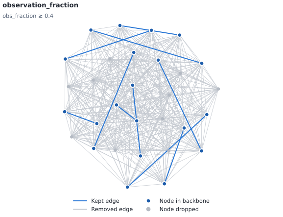
Backbone (blue) over the original graph (gray). Kept 10 of 382 edges (3%) and 20 of 30 nodes.#
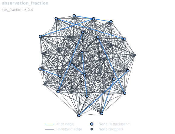
Backbone (blue) over the original graph (gray). Kept 10 of 382 edges (3%) and 20 of 30 nodes.#
persistence() on 20 synthetic snapshots, keeping persistence ≥ 0.8.
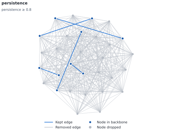
Backbone (blue) over the original graph (gray). Kept 5 of 382 edges (1%) and 10 of 30 nodes.#
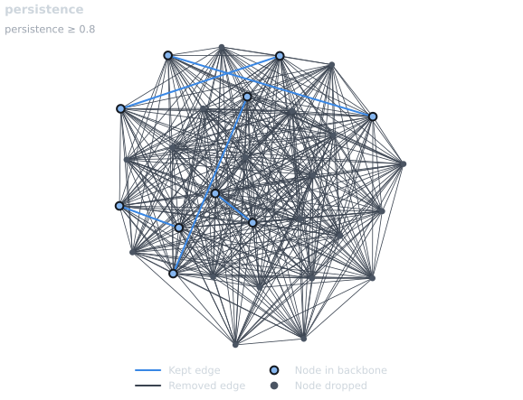
Backbone (blue) over the original graph (gray). Kept 5 of 382 edges (1%) and 10 of 30 nodes.#
backbone_stability() on 20 synthetic snapshots, keeping stability ≥ 0.3.
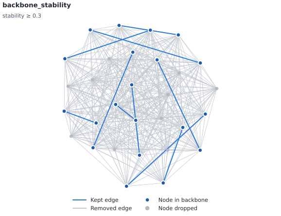
Backbone (blue) over the original graph (gray). Kept 10 of 382 edges (3%) and 20 of 30 nodes.#
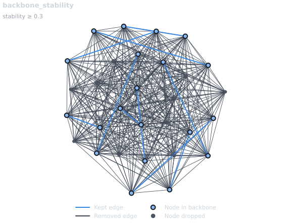
Backbone (blue) over the original graph (gray). Kept 10 of 382 edges (3%) and 20 of 30 nodes.#
weight_trend() on 20 synthetic snapshots, keeping weight_mean ≥ 3.
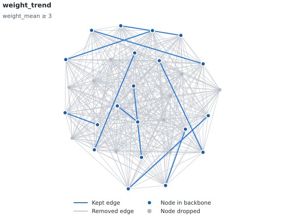
Backbone (blue) over the original graph (gray). Kept 10 of 382 edges (3%) and 20 of 30 nodes.#
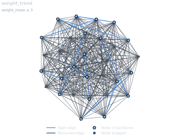
Backbone (blue) over the original graph (gray). Kept 10 of 382 edges (3%) and 20 of 30 nodes.#
edge_persistence_hmm() on 20 synthetic snapshots, keeping hmm_keep (min_steps=8).
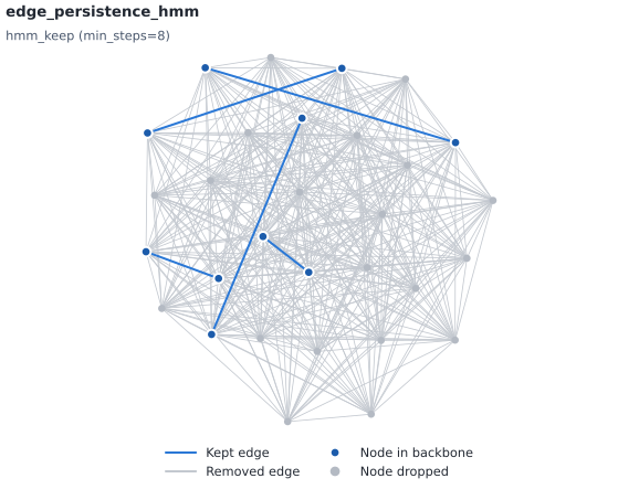
Backbone (blue) over the original graph (gray). Kept 5 of 382 edges (1%) and 10 of 30 nodes.#
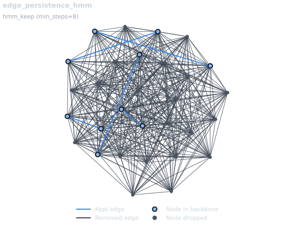
Backbone (blue) over the original graph (gray). Kept 5 of 382 edges (1%) and 10 of 30 nodes.#
kalman_backbone() on 20 synthetic snapshots, keeping kalman_pvalue < 0.05 (disparity_filter per step).
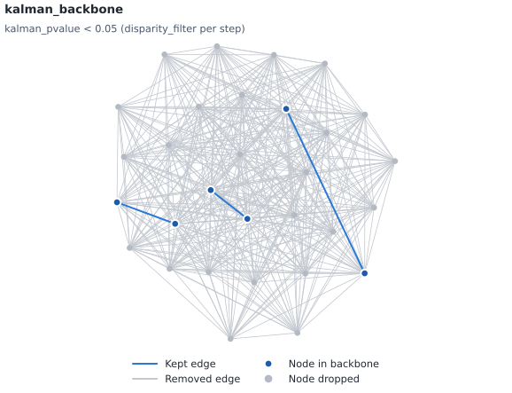
Backbone (blue) over the original graph (gray). Kept 3 of 382 edges (1%) and 6 of 30 nodes.#
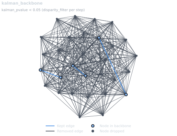
Backbone (blue) over the original graph (gray). Kept 3 of 382 edges (1%) and 6 of 30 nodes.#
Forms
- nx_backbone.temporal_form(T, time='time', start='start', end='end')[source]#
Return the form of a temporal network: snapshots, events, or spans.
- Parameters:
- Tdict, list, MultiGraph or MultiDiGraph
Snapshots (a dict
{time: graph}or a list of graphs), or a multigraph of events or spans.- timestr or None, optional (default=”time”)
Edge attribute holding an event’s time.
Nonenever reads T as events.- start, endstr or None, optional (default=”start”, “end”)
Edge attributes holding a span’s start and end.
Nonenever reads T as spans.
- Returns:
- form{“snapshots”, “events”, “spans”}
"events"when every edge has a time,"spans"when every edge has a start and an end. A multigraph without edges is read from itsgraph["temporal"]record when it has one.
- Raises:
- TypeError
If T is neither a graph nor a dict or list of graphs, or a snapshot is not a graph.
- ValueError
If there are no snapshots, or a snapshot time is missing.
- NetworkXError
If T is a simple graph; if its edges have both the event and the span attributes, or neither on every edge, or (no edges) its form is unknown; or if snapshots mix directed and undirected graphs.
- NetworkXNotImplemented
If a snapshot is a multigraph.
See also
Examples
>>> import networkx as nx
>>> from nx_backbone import temporal_form
>>> temporal_form([nx.path_graph(3), nx.path_graph(4)])
'snapshots'
>>> M = nx.MultiGraph([(0, 1, {"time": 3}), (0, 1, {"time": 5})])
>>> temporal_form(M)
'events'
>>> M = nx.MultiGraph([(0, 1, {"t0": 3, "t1": 7})])
>>> temporal_form(M, start="t0", end="t1")
'spans'
Computational complexity estimate is
O(m + S log S)time andO(S)space.
- nx_backbone.convert_temporal(T, to, **kwargs)[source]#
Convert a temporal network to snapshots, events, or spans.
Detects the form of T with
temporal_form()and calls the matching converter.- Parameters:
- Tdict, list, MultiGraph or MultiDiGraph
Snapshots, events, or spans.
- to{“snapshots”, “events”, “spans”}
The form to return.
- **kwargs
Passed to the converter:
snapshots_from_events(),snapshots_from_spans(),events_from_snapshots(),spans_from_snapshots(),events_from_spans()orspans_from_events().time,startandendalso name the attributes used to detect the form.
- Returns:
- converteddict, MultiGraph or MultiDiGraph
T in the requested form. If T is already in that form, a copy (snapshots as a dict of graph copies).
- Raises:
- ValueError
If to is not a known form.
- TypeError
If kwargs are given but T is already in the requested form, or the converter does not take them.
See also
Examples
>>> import networkx as nx
>>> from nx_backbone import convert_temporal
>>> M = nx.MultiGraph([(0, 1, {"time": 0}), (0, 1, {"time": 3})])
>>> S = convert_temporal(M, to="snapshots", freq=2)
>>> {t: G.number_of_edges() for t, G in S.items()}
{0: 1, 2: 1}
>>> spans = convert_temporal(M, to="spans", duration=1)
>>> sorted((d["start"], d["end"]) for *_, d in spans.edges(data=True))
[(0, 1), (3, 4)]
Computational complexity estimate is
that of the convertertime andthat of the converterspace.
Collapsing to a static graph
- nx_backbone.flatten_temporal(T, weight='weight', aggregate='sum', window=None, time='time', start='start', end='end')[source]#
Collapse a temporal network into one static weighted graph.
Every observation of a node pair (an edge in a snapshot, an event, or a span) is combined into a single edge whose
weightaggregates the observations’ weights, and which records how often and when the pair was observed. The result is an ordinaryGraphorDiGraph, so any static backbone method applies to it.- Parameters:
- Tdict, list, MultiGraph or MultiDiGraph
Snapshots, events, or spans (see
temporal_form()).- weightstr, optional (default=”weight”)
Edge attribute holding each observation’s weight; a missing weight counts as 1. The aggregated value is stored under the same name.
- aggregate{“sum”, “count”, “max”, “min”, “mean”, “duration”}, optional
How the observations’ weights combine, as in
multigraph_to_weighted();"count"gives the number of observations."duration"(spans only) gives the total time the pair is in contact: the length of the union of its spans within window, so overlapping spans are not counted twice. Default"sum".- windowtuple (t0, t1) or None, optional (default=None)
Keep only what happens in the half-open interval
[t0, t1); either bound may beNonefor an open end. Snapshots and events are kept when their time falls in the window; spans are clipped to it (a span withstart == endis kept when its start falls in the window).- timestr, optional (default=”time”)
Edge attribute holding an event’s time.
- start, endstr, optional (default=”start”, “end”)
Edge attributes holding a span’s start and end.
- Returns:
- HGraph or DiGraph
One edge per node pair observed in the window, with:
weight: the aggregated weight;
n_obs: the number of observations (snapshots containing the edge, events, or spans);firstandlast: the earliest and latest observation times (for spans, the earliest clipped start and the latest clipped end);active_time(spans only): the length of the union of the pair’s clipped spans;the attributes that all of the pair’s observations share.
Nodes are those present in the window, with their attributes (from the latest snapshot that holds them, or from T); without a window every node of T is kept, including isolated nodes. The graph attributes come from the latest snapshot in the window (or from T), and
H.graph["temporal"]records the input form, aggregate, window, and the first and last observation times.
- Raises:
- ValueError
If aggregate is unknown,
"duration"is used with snapshots or events, or window is empty.- TypeError
If window is not a pair, or times cannot be compared with it.
- NetworkXError
If T is not a temporal network (see
temporal_form()).
Notes
To collapse at a coarser resolution, bin first and then flatten: for example
flatten_temporal(snapshots_from_events(M, freq=7))counts the weeks in which a pair interacts, whereflatten_temporal(M, aggregate="count")counts its events.The result drops the order and timing of the observations beyond
first,lastandactive_time; use the temporal filters to score edges by how they behave over time.Examples
>>> import networkx as nx
>>> from nx_backbone import flatten_temporal
>>> G1 = nx.Graph([("a", "b", {"weight": 2}), ("b", "c", {"weight": 1})])
>>> G2 = nx.Graph([("a", "b", {"weight": 3})])
>>> H = flatten_temporal({0: G1, 1: G2})
>>> H["a"]["b"]
{'weight': 5, 'n_obs': 2, 'first': 0, 'last': 1}
>>> flatten_temporal({0: G1, 1: G2}, aggregate="mean")["a"]["b"]["weight"]
2.5
Spans can be weighted by how long the pair is in contact:
>>> M = nx.MultiGraph()
>>> M.add_edges_from([("a", "b", {"start": 0, "end": 4.5}),
...                   ("a", "b", {"start": 9, "end": 9.5})])
[0, 1]
>>> H = flatten_temporal(M, aggregate="duration")
>>> H["a"]["b"]["weight"], H["a"]["b"]["n_obs"]
(5.0, 2)
>>> flatten_temporal(M, aggregate="duration", window=(2, 10))["a"]["b"]["weight"]
3.0
Computational complexity estimate is
O(n + m + S log S)time andO(n + m)space.
Binning events and spans into snapshots
- nx_backbone.snapshots_from_events(M, time='time', freq=None, origin=None, weight='weight', aggregate='sum')[source]#
Bin timestamped events into snapshots.
- Parameters:
- MMultiGraph or MultiDiGraph
One edge per event, with its time in the time attribute.
- timestr, optional (default=”time”)
Edge attribute holding each event’s time.
- freqnumber, timedelta, str or None, optional (default=None)
Width of each bin: a number for numeric times, a
datetime.timedeltaor a pandas frequency string such as"1D"for datetimes.Nonemakes one snapshot per distinct time.- origintime or None, optional (default=None)
Start of bin 0 (default: the earliest time). Only used with freq.
- weightstr, optional (default=”weight”)
Edge attribute combined across the events of a node pair in one bin.
- aggregate{“sum”, “count”, “max”, “min”, “mean”}, optional (default=”sum”)
How those weights combine, as in
multigraph_to_weighted().
- Returns:
- snapshotsdict
{bin start: Graph or DiGraph}in time order, from the first to the last bin with an event, empty bins included. Each graph has the nodes with an event in its bin (with their attributes from M) and M’s graph attributes. Each edge hasweight,edge_count(the number of events) and the attributes its events share. If M carries agraph["temporal"]record fromevents_from_snapshots()and freq and origin areNone, the original snapshots are returned instead (see Notes).
- Raises:
- NetworkXNotImplemented
If M is not a multigraph.
- ValueError
If an event has no time, freq is not positive, origin is given without freq, or aggregate is unknown.
- TypeError
If the times and freq cannot be combined.
- ImportError
If freq is a string and pandas is not installed.
Notes
Bin
kis the half-open interval[origin + k * freq, origin + (k + 1) * freq). For a calendar frequency such as"MS"(pandas only), bins step by calendar periods from origin.Lossless round trip:
snapshots_from_events(events_from_snapshots(S))returns S as a dict (up to the order of edges), with its empty snapshots, isolated nodes, and node, edge and graph attributes, by reading thegraph["temporal"]record. The record is ignored when an event’s time is not a recorded snapshot time or a node pair has two events at one time.Lossy direction: binning drops the event-level detail (each pair keeps one edge per bin), nodes without an event in a bin, and the attributes the events of a bin do not share;
weightandedge_countare added.Examples
>>> import networkx as nx
>>> from nx_backbone import snapshots_from_events
>>> M = nx.MultiGraph()
>>> M.add_edges_from([("a", "b", {"time": 0}), ("a", "b", {"time": 1}),
...                   ("b", "c", {"time": 5})])
[0, 1, 0]
>>> S = snapshots_from_events(M, freq=2)
>>> {t: sorted(G.edges(data="weight")) for t, G in S.items()}
{0: [('a', 'b', 2)], 2: [], 4: [('b', 'c', 1)]}
Without freq, every distinct time is a snapshot:
>>> sorted(snapshots_from_events(M))
[0, 1, 5]
Computational complexity estimate is
O(n + m log m + B)time andO(n + m + B)space.
- nx_backbone.snapshots_from_spans(M, start='start', end='end', freq=None, origin=None, weight='weight', aggregate='sum')[source]#
Bin spans (contacts with a start and an end) into snapshots.
- Parameters:
- MMultiGraph or MultiDiGraph
One edge per span, covering
[start, end).- start, endstr, optional (default=”start”, “end”)
Edge attributes holding each span’s start and end.
- freqnumber, timedelta, str or None, optional (default=None)
Width of each bin (see
snapshots_from_events()).Nonemakes one snapshot per interval between consecutive distinct start or end times, so each snapshot holds exactly the spans active throughout it.- origintime or None, optional (default=None)
Start of bin 0 (default: the earliest start). Only used with freq.
- weightstr, optional (default=”weight”)
Edge attribute combined across the spans of a node pair in one bin.
- aggregate{“sum”, “count”, “max”, “min”, “mean”}, optional (default=”sum”)
How those weights combine, as in
multigraph_to_weighted().
- Returns:
- snapshotsdict
{bin start: Graph or DiGraph}in time order, from the first to the last bin a span overlaps, empty bins included. A span is observed in every bin it overlaps; a span withstart == endonly in the bin holding its start. Nodes, edges and attributes are as insnapshots_from_events(). With agraph["temporal"]record fromspans_from_snapshots()and no freq or origin, the original snapshots are returned.
- Raises:
- NetworkXNotImplemented
If M is not a multigraph.
- ValueError
If a span has no start or end or ends before it starts, freq is not positive, origin is given without freq, or aggregate is unknown.
- TypeError
If the times and freq cannot be combined.
- ImportError
If freq is a string and pandas is not installed.
Notes
A span’s weight is not split across the bins it overlaps: a span of weight 3 adds 3 to each of them.
Lossless round trip:
snapshots_from_spans(spans_from_snapshots(S))returns S as a dict (up to the order of edges), using thegraph["temporal"]record. Lossy direction: as forsnapshots_from_events().Examples
>>> import networkx as nx
>>> from nx_backbone import snapshots_from_spans
>>> M = nx.MultiGraph()
>>> M.add_edges_from([("a", "b", {"start": 0, "end": 5}),
...                   ("b", "c", {"start": 3, "end": 4})])
[0, 0]
>>> S = snapshots_from_spans(M, freq=2)
>>> {t: sorted(G.edges) for t, G in S.items()}
{0: [('a', 'b')], 2: [('a', 'b'), ('b', 'c')], 4: [('a', 'b')]}
Without freq, snapshots start wherever a span starts or ends:
>>> {t: sorted(G.edges) for t, G in snapshots_from_spans(M).items()}
{0: [('a', 'b')], 3: [('a', 'b'), ('b', 'c')], 4: [('a', 'b')]}
Computational complexity estimate is
O(n + m log m + m_B + B)time andO(n + m_B + B)space.
Snapshots to events and spans
- nx_backbone.events_from_snapshots(S, time='time')[source]#
Return one event per edge per snapshot.
- Parameters:
- Sdict or list of graphs
Snapshots:
{time: Graph or DiGraph}, or a list read as times0, ..., T - 1.- timestr, optional (default=”time”)
Edge attribute that stores each event’s time (its snapshot’s key).
- Returns:
- MMultiGraph or MultiDiGraph
One edge per snapshot edge, with that edge’s attributes and its time. M has every node of every snapshot (isolated ones too), with its attributes from the latest snapshot that holds it, and the last snapshot’s graph attributes, plus the
M.graph["temporal"]record that makes the conversion reversible.
- Raises:
- TypeError
If S is not a dict or list of graphs, or its times are not comparable.
- ValueError
If S is empty, a time is missing, or an edge already has a time attribute.
- NetworkXError
If the snapshots mix directed and undirected graphs.
- NetworkXNotImplemented
If a snapshot is a multigraph.
Notes
Lossless:
snapshots_from_events()with no freq returns S (as a dict) from M’sgraph["temporal"]record, including empty snapshots, isolated nodes and per-snapshot node and graph attributes. Without the record (for example afterto_event_table()), the events alone keep the edges, their attributes and times, and the nodes, but not empty snapshots, isolated nodes per snapshot, or per-snapshot attributes.Examples
>>> import networkx as nx
>>> from nx_backbone import events_from_snapshots, snapshots_from_events
>>> S = {2020: nx.Graph([("a", "b")]), 2021: nx.Graph([("a", "b"), ("b", "c")])}
>>> M = events_from_snapshots(S)
>>> sorted((u, v, t) for u, v, t in M.edges(data="time"))
[('a', 'b', 2020), ('a', 'b', 2021), ('b', 'c', 2021)]
>>> R = snapshots_from_events(M)
>>> all(nx.utils.graphs_equal(R[t], S[t]) for t in S)
True
Computational complexity estimate is
O(S log S + n_S + m_S)time andO(n_S + m_S)space.
- nx_backbone.spans_from_snapshots(S, start='start', end='end', freq=None, end_time=None)[source]#
Merge each edge’s runs of consecutive snapshots into spans.
- Parameters:
- Sdict or list of graphs
Snapshots:
{time: Graph or DiGraph}, or a list read as times0, ..., T - 1.- start, endstr, optional (default=”start”, “end”)
Edge attributes that store each span’s start and end.
- freqnumber, timedelta, str or None, optional (default=None)
Length of the last snapshot: it ends at its time plus freq.
- end_timetime or None, optional (default=None)
When the last snapshot ends, instead of freq.
- Returns:
- MMultiGraph or MultiDiGraph
One edge per run: a maximal sequence of consecutive snapshots in which the edge is present with the same attributes. The span starts at the run’s first snapshot time and ends at the time of the snapshot after the run (half-open, so it covers the run’s snapshots and no other); a run reaching the last snapshot ends when that snapshot ends. Nodes, graph attributes and the
M.graph["temporal"]record are as inevents_from_snapshots(); the record also stores"end_time".
- Raises:
- TypeError
If S is not a dict or list of graphs, or its times are not comparable.
- ValueError
If S is empty, a time is missing, an edge already has a start or end attribute, or the end of the last snapshot cannot be determined.
- NetworkXError
If the snapshots mix directed and undirected graphs.
- NetworkXNotImplemented
If a snapshot is a multigraph.
- ImportError
If freq is a string and pandas is not installed.
Notes
The last snapshot ends at end_time if given, else at its time plus freq, else one step later when S is a list (times
0, ..., T - 1) or its times are evenly spaced. Otherwise (uneven times, or a single snapshot in a dict) aValueErrorasks for freq or end_time.Lossless:
snapshots_from_spans()with no freq returns S from the record. Splitting runs where an edge’s attributes change keeps each snapshot’s edge attributes, so the spans alone keep the edges, their attributes and when they were present.Examples
>>> import networkx as nx
>>> from nx_backbone import spans_from_snapshots, snapshots_from_spans
>>> S = [nx.Graph([(0, 1)]), nx.Graph([(0, 1), (1, 2)]), nx.Graph([(1, 2)])]
>>> M = spans_from_snapshots(S)
>>> sorted((u, v, d["start"], d["end"]) for u, v, d in M.edges(data=True))
[(0, 1, 0, 2), (1, 2, 1, 3)]
>>> R = snapshots_from_spans(M)
>>> all(nx.utils.graphs_equal(R[t], S[t]) for t in range(3))
True
Computational complexity estimate is
O(S log S + n_S + m_S)time andO(n_S + m_S)space.
Between events and spans
- nx_backbone.events_from_spans(M, start='start', end='end', time='time', freq=None, origin=None)[source]#
Turn spans into events: one at each span’s start, or one per bin.
- Parameters:
- MMultiGraph or MultiDiGraph
One edge per span, covering
[start, end).- start, endstr, optional (default=”start”, “end”)
Edge attributes holding each span’s start and end.
- timestr, optional (default=”time”)
Edge attribute that stores each event’s time.
- freqnumber, timedelta, str or None, optional (default=None)
Nonemakes one event per span, at its start. Otherwise, one event per bin the span overlaps, at the bin’s start, with the bins ofsnapshots_from_spans().- origintime or None, optional (default=None)
Start of bin 0 (default: the earliest start). Only used with freq.
- Returns:
- eventsMultiGraph or MultiDiGraph
Same class, nodes and graph attributes as M (without a
graph["temporal"]record). Each event has its span’s attributes except start and end.
- Raises:
- NetworkXNotImplemented
If M is not a multigraph.
- ValueError
If a span has no start or end or ends before it starts, a span already has a time attribute, freq is not positive, or origin is given without freq.
- TypeError
If the times and freq cannot be combined.
- ImportError
If freq is a string and pandas is not installed.
Notes
An event is instantaneous and a span is not, so no choice keeps everything. The two choices here each keep one well-defined thing:
freq=Nonekeeps when each contact began (onset events), the usual reading of contact data as events. Durations are lost.With freq, binning the events with the same freq and origin gives the same snapshots, weights included, as binning the spans:
snapshots_from_events(events_from_spans(M, freq=f), freq=f)equalssnapshots_from_spans(M, freq=f). Times within a bin are lost.
Examples
>>> import networkx as nx
>>> from nx_backbone import events_from_spans
>>> M = nx.MultiGraph([("a", "b", {"start": 1, "end": 6})])
>>> [t for *_, t in events_from_spans(M).edges(data="time")]
[1]
>>> [t for *_, t in events_from_spans(M, freq=2, origin=0).edges(data="time")]
[0, 2, 4]
Computational complexity estimate is
O(n + m log B + m_B)time andO(n + m_B)space.
- nx_backbone.spans_from_events(M, time='time', start='start', end='end', *, duration, gap=0, weight='weight', aggregate='sum')[source]#
Turn events into spans: each lasts duration, and close ones merge.
- Parameters:
- MMultiGraph or MultiDiGraph
One edge per event, with its time in the time attribute.
- timestr, optional (default=”time”)
Edge attribute holding each event’s time.
- start, endstr, optional (default=”start”, “end”)
Edge attributes that store each span’s start and end.
- durationnumber, timedelta or str
How long each event lasts: an event at
tcovers[t, t + duration).0makes instantaneous spans.- gapnumber, timedelta, str or None, optional (default=0)
Events of the same node pair merge into one span when the next one starts no later than gap after the current span ends;
0merges overlapping and touching spans.Nonenever merges.- weightstr, optional (default=”weight”)
Edge attribute combined across the events of a span.
- aggregate{“sum”, “count”, “max”, “min”, “mean”}, optional (default=”sum”)
How those weights combine, as in
multigraph_to_weighted().
- Returns:
- spansMultiGraph or MultiDiGraph
Same class, nodes and graph attributes as M (without a
graph["temporal"]record). Each span runs from its first event’s time to its last event’s time plus duration, and hasweight,edge_count(its number of events) and the attributes its events share.
- Raises:
- NetworkXNotImplemented
If M is not a multigraph.
- ValueError
If an event has no time, duration or gap is negative, or aggregate is unknown.
- TypeError
If the times and duration or gap cannot be combined.
- ImportError
If duration or gap is a string and pandas is not installed.
Notes
Lossy: event times inside a merged span, and the attributes its events do not share, are lost. With
gap=Noneeach event becomes its own span, andevents_from_spans()gives back the event times.Examples
>>> import networkx as nx
>>> from nx_backbone import spans_from_events
>>> M = nx.MultiGraph()
>>> M.add_edges_from([("a", "b", {"time": 0}), ("a", "b", {"time": 1}),
...                   ("a", "b", {"time": 9})])
[0, 1, 2]
>>> S = spans_from_events(M, duration=2)
>>> sorted((d["start"], d["end"], d["weight"]) for *_, d in S.edges(data=True))
[(0, 3, 2), (9, 11, 1)]
Computational complexity estimate is
O(n + m log m)time andO(n + m)space.
pandas event tables
- nx_backbone.from_event_table(df, source='source', target='target', time='time', end=None, weight=None, directed=False, edge_attrs=None)[source]#
Return events (or spans) from a pandas table with one row per event.
- Parameters:
- dfpandas.DataFrame
One row per event (or span).
- source, targetstr, optional (default=”source”, “target”)
Columns holding the two endpoints.
- timestr, optional (default=”time”)
Column holding each event’s time, or each span’s start when end is given. It becomes the edge attribute of the same name.
- endstr or None, optional (default=None)
Column holding each span’s end. If given, the result is spans with
start=timeandend=end.- weightstr or None, optional (default=None)
Column copied to the edge attribute of the same name.
- directedbool, optional (default=False)
Return a
MultiDiGraph(sourcetotarget) instead of aMultiGraph.- edge_attrsbool, sequence of str or None, optional (default=None)
Further columns to copy as edge attributes;
Truecopies every other column.
- Returns:
- MMultiGraph or MultiDiGraph
One edge per row, in row order, with the time (and end) attribute and the copied columns. A missing value (
NaN,None,NaT) in a copied column leaves that attribute off the edge.
- Raises:
- TypeError
If df is not a pandas
DataFrame.- ValueError
If a named column is missing, an endpoint, time or end is missing, or a span ends before it starts.
Notes
Duplicate rows are kept as parallel edges: two identical rows are two events, which
snapshots_from_events()adds up when it bins them. (to_graph()refuses duplicates instead, because a simple graph would silently drop them.) Values come fromSeries.tolist(), so datetime columns give pandasTimestamptimes.Examples
>>> import pandas as pd
>>> from nx_backbone import from_event_table
>>> df = pd.DataFrame({"source": ["a", "a", "b"], "target": ["b", "b", "c"],
...                    "time": [0, 1, 5], "w": [2, 3, 1]})
>>> M = from_event_table(df, weight="w")
>>> sorted(M.edges(data=True))
[('a', 'b', {'time': 0, 'w': 2}), ('a', 'b', {'time': 1, 'w': 3}), ('b', 'c', {'time': 5, 'w': 1})]
Computational complexity estimate is
O(r)time andO(r)space.
- nx_backbone.to_event_table(T, source='source', target='target', time='time', start='start', end='end', edge_attrs=True)[source]#
Return events or spans as a pandas table with one row per edge.
- Parameters:
- Tdict, list, MultiGraph or MultiDiGraph
Events, spans, or snapshots (written as the events of
events_from_snapshots()).- source, targetstr, optional (default=”source”, “target”)
Columns for the two endpoints.
- timestr, optional (default=”time”)
Edge attribute (and column) holding an event’s time.
- start, endstr, optional (default=”start”, “end”)
Edge attributes (and columns) holding a span’s start and end.
- edge_attrsbool or sequence of str, optional (default=True)
Edge attributes to write as further columns:
Truefor all,Falsefor none, or a list of names.
- Returns:
- dfpandas.DataFrame
Columns source, target, then time (events) or start and end (spans), then the edge attributes in order of first appearance. Rows are sorted by time (stable). An attribute an edge lacks is
NaN.
- Raises:
- ImportError
If pandas is not installed.
- ValueError
If an edge attribute is named like the source or target column.
See also
Notes
from_event_table(to_event_table(M), weight=..., edge_attrs=True)gives back the events or spans of M: endpoints, times, ends and edge attributes (an integer column with a missing value becomes float). Node attributes, isolated nodes, graph attributes and thegraph["temporal"]record are not written.Examples
>>> import networkx as nx
>>> from nx_backbone import to_event_table
>>> M = nx.MultiGraph([("b", "c", {"time": 5}), ("a", "b", {"time": 0, "w": 2})])
>>> to_event_table(M)
  source target  time    w
0      a      b     0  2.0
1      b      c     5  NaN
Computational complexity estimate is
O(m log m)time andO(m)space.