Temporal backbones, from snapshots to smoothing

A network observed over time is not one network but many: who emailed whom each week, which stations exchanged passengers each hour, which proteins were seen together in each experiment. A temporal backbone keeps the ties that matter over time, and “matter” can mean several things: ties that are seen often, ties that last, ties that a static backbone keeps again and again, or ties whose weight is significant once the noise of single observations is averaged out.

This tutorial follows that question from the raw records to a backbone:

1. three ways to record time (snapshots, events and spans) and binning;

2. collapsing time into one static graph, and what that hides;

3. descriptive scores: how often, how steadily, and how often a static backbone keeps an edge;

4. smoothing per-step significance with a Kalman filter, and its risks;

5. a hidden Markov model of persistent activity;

6. choosing among them.

Every number and figure below is computed when the documentation is built, from small seeded synthetic networks. For the calls themselves, score by score, see the short how-to tutorial Temporal Backbones; for every format conversion, see the user guide Temporal networks: formats and conversions.

Setting up

The temporal functions need only NetworkX for the conversions and the descriptive scores; weight_trend() and the two model-based methods also need NumPy, and kalman_backbone() needs SciPy.

import math
import random
import warnings
from itertools import combinations
from pathlib import Path

import matplotlib.pyplot as plt
import networkx as nx
import numpy as np
from _figures import style
from matplotlib.collections import PatchCollection
from matplotlib.lines import Line2D
from matplotlib.patches import Patch, Rectangle

import nx_backbone as nb



def table(header, rows):
    """Print rows as an aligned plain-text table."""
    rows = [[str(c) for c in row] for row in [header, *rows]]
    widths = [max(len(r[i]) for r in rows) for i in range(len(header))]
    for k, row in enumerate(rows):
        print("  ".join(c.ljust(w) for c, w in zip(row, widths)).rstrip())
        if k == 0:
            print("  ".join("-" * w for w in widths))


def key(u, v):
    """An undirected edge as a sorted tuple."""
    return (u, v) if u <= v else (v, u)

Three ways to record time

Suppose four people wear proximity badges for an eight-hour day. The badges log spans: contacts with a start and an end time. Many systems log something else. A message log has events, one per contact with a single timestamp and no duration. A survey repeated every hour has snapshots, one ordinary graph per time step. nx_backbone.temporal accepts all three, built from ordinary NetworkX graphs: snapshots are a dict {time: graph}, events a MultiGraph with a time on every edge, and spans a multigraph with start and end.

Here is the badge log, in hours. Ann and Bob meet briefly and often, Bob and Cat once for most of the day, Cat and Dan twice for a while, and Ann and Dan once, briefly.

CONTACTS = {
    ("ann", "bob"): [
        (0.2, 0.5),
        (1.1, 1.4),
        (2.0, 2.2),
        (3.4, 3.7),
        (4.5, 4.8),
        (6.1, 6.3),
        (7.2, 7.5),
    ],
    ("bob", "cat"): [(1.0, 6.5)],
    ("cat", "dan"): [(0.5, 2.0), (5.0, 7.5)],
    ("ann", "dan"): [(3.0, 3.5)],
}
PAIRS = list(CONTACTS)

spans = nx.MultiGraph()
for (u, v), contacts in CONTACTS.items():
    for start, end in contacts:
        spans.add_edge(u, v, start=start, end=end)

The converters move between the forms. Keeping only each contact’s onset gives events; binning with a step width freq= gives snapshots, one per bin, in which a pair is present if any of its spans overlaps the bin. origin=0 starts the bins on the hour.

events = nb.events_from_spans(spans)
hourly = nb.snapshots_from_spans(spans, freq=1, origin=0)
two_hourly = nb.snapshots_from_spans(spans, freq=2, origin=0)

print(
    "Forms:",
    nb.temporal_form(spans),
    nb.temporal_form(events),
    nb.temporal_form(hourly),
)
print(
    f"{events.number_of_edges()} events, {len(hourly)} hourly snapshots, "
    f"{len(two_hourly)} two-hourly snapshots"
)

Forms: spans events snapshots
11 events, 8 hourly snapshots, 4 two-hourly snapshots

Binning the events instead of the spans loses the durations: an event marks only the bin of its onset, so the day-long contact of Bob and Cat appears in one hourly snapshot rather than in every hour it covers.

from_events = nb.snapshots_from_events(events, freq=1, origin=0)
for name, snaps in (("spans", hourly), ("events", from_events)):
    steps = [t for t, G in snaps.items() if G.has_edge("bob", "cat")]
    print(f"Bob-Cat present in the hourly snapshots binned from {name}: {steps}")

Bob-Cat present in the hourly snapshots binned from spans: [1, 2, 3, 4, 5, 6]
Bob-Cat present in the hourly snapshots binned from events: [1]

The figure lays the four records side by side on one time axis.

T_END = 8


def draw_forms(mode):
    p = style.palette(mode)
    fig, axes = plt.subplots(
        4, 1, figsize=(7.2, 6.0), sharex=True, gridspec_kw={"hspace": 0.55}
    )
    rows = {pair: i for i, pair in enumerate(reversed(PAIRS))}
    labels = [f"{u}–{v}" for u, v in reversed(PAIRS)]
    ax = axes[0]
    for u, v, t in events.edges(data="time"):
        y = rows[(u, v)] if (u, v) in rows else rows[(v, u)]
        ax.plot([t, t], [y - 0.32, y + 0.32], color=p.kept, lw=1.8)
    ax.set_title("Events: one timestamp per contact (onsets)")
    ax = axes[1]
    for u, v, d in spans.edges(data=True):
        y = rows[(u, v)] if (u, v) in rows else rows[(v, u)]
        ax.add_patch(
            Rectangle(
                (d["start"], y - 0.3),
                d["end"] - d["start"],
                0.6,
                facecolor=p.kept,
                linewidth=0,
            )
        )
    ax.set_title("Spans: a start and an end per contact")
    for ax, snaps, width, title in (
        (axes[2], hourly, 1, "Snapshots: spans binned with freq=1 (hours)"),
        (axes[3], two_hourly, 2, "Snapshots: spans binned with freq=2"),
    ):
        for t, G in snaps.items():
            for u, v in G.edges():
                y = rows[(u, v)] if (u, v) in rows else rows[(v, u)]
                ax.add_patch(
                    Rectangle(
                        (t + 0.06, y - 0.3),
                        width - 0.12,
                        0.6,
                        facecolor=p.kept,
                        linewidth=0,
                    )
                )
        for t in snaps:
            ax.axvline(t, color=p.hairline, lw=0.75, zorder=0)
        ax.set_title(title)
    for ax in axes:
        ax.set_yticks(range(len(labels)), labels)
        ax.set_ylim(-0.6, len(labels) - 0.4)
        ax.set_xlim(0, T_END)
        ax.tick_params(axis="y", length=0)
        ax.spines["left"].set_visible(False)
    axes[-1].set_xlabel("Time (hours)")
    axes[-1].set_xticks(range(T_END + 1))
    return fig


save("temporal_forms", draw_forms)

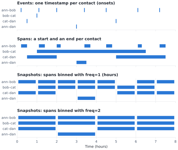
The same badge log as events (onsets only), spans, and snapshots binned at one and two hours. Wider bins merge contacts and make brief and long contacts look alike.

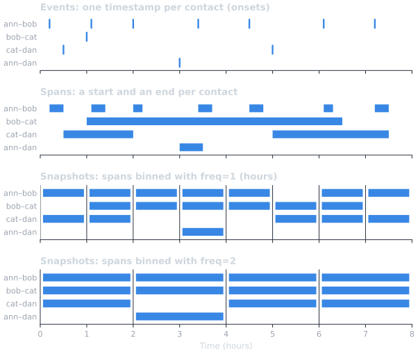
The same badge log as events (onsets only), spans, and snapshots binned at one and two hours. Wider bins merge contacts and make brief and long contacts look alike.

The conversions between snapshots and events or spans are lossless; binning is not (see the table in Temporal networks: formats and conversions). The bin width is a modeling choice: it sets what “at the same time” means.

Collapsing time

The quickest way to a backbone is to forget time altogether. flatten_temporal() collapses any of the three forms into one static weighted graph, with one edge per pair, so every static backbone method applies. The weight depends on aggregate=: counting contacts and adding up their durations tell different stories about the same day.

by_count = nb.flatten_temporal(spans, aggregate="count")
by_duration = nb.flatten_temporal(spans, aggregate="duration")
table(
    ["Pair", "Contacts (count)", "Hours in contact (duration)"],
    [
        [
            f"{u}–{v}",
            by_count[u][v]["weight"],
            f"{by_duration[u][v]['weight']:.1f}",
        ]
        for u, v in PAIRS
    ],
)


def heaviest(H):
    return max(H.edges, key=lambda e: H.edges[e]["weight"])


print("Heaviest pair by count:", "–".join(heaviest(by_count)))
print("Heaviest pair by duration:", "–".join(heaviest(by_duration)))



def draw_flatten(mode):
    p = style.palette(mode)
    fig, axes = plt.subplots(1, 2, figsize=(7.2, 2.2), sharey=True)
    labels = [f"{u}–{v}" for u, v in PAIRS]
    ys = range(len(PAIRS))
    for ax, H, title, fmt in (
        (axes[0], by_count, "Weight = number of contacts", "{:.0f}"),
        (axes[1], by_duration, "Weight = hours in contact", "{:.1f}"),
    ):
        values = [H[u][v]["weight"] for u, v in PAIRS]
        ax.barh(ys, values, height=0.55, color=p.kept)
        for y, value in zip(ys, values):
            ax.text(
                value,
                y,
                " " + fmt.format(value),
                va="center",
                ha="left",
                color=p.ink,
                fontsize=8.5,
            )
        ax.set_title(title)
        ax.set_xlim(0, max(values) * 1.25)
        ax.set_xticks([])
        ax.spines["bottom"].set_visible(False)
        ax.spines["left"].set_visible(False)
        ax.tick_params(axis="y", length=0)
    axes[0].set_yticks(list(ys), labels)
    axes[0].invert_yaxis()
    fig.tight_layout()
    return fig


save("temporal_flatten", draw_flatten)

Pair     Contacts (count)  Hours in contact (duration)
-------  ----------------  ---------------------------
ann–bob  7                 1.9
bob–cat  1                 5.5
cat–dan  2                 4.0
ann–dan  1                 0.5
Heaviest pair by count: ann–bob
Heaviest pair by duration: bob–cat

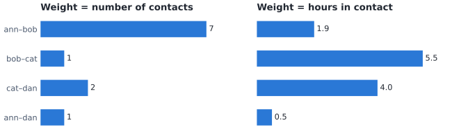
The badge log flattened two ways. The order of the pairs depends on whether a weight counts contacts or time in contact.

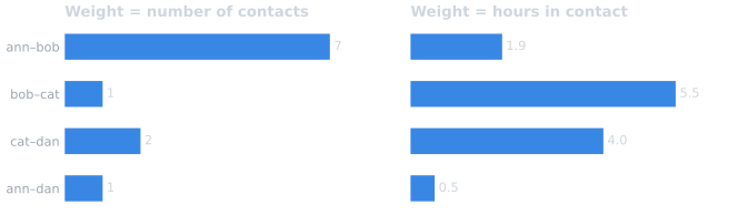
The badge log flattened two ways. The order of the pairs depends on whether a weight counts contacts or time in contact.

Neither weight is wrong; they answer different questions. Decide what a unit of weight should mean before choosing a static method, since several null models assume the weights are counts (see Statistical null models side by side).

What flattening hides

Flattening keeps how much, but not when. To see what that costs, we need a longer record. The rest of this tutorial uses two synthetic networks; the first is a sequence of snapshots of 30 people, all present in every one of 24 steps, with three kinds of edges:

• a persistent block: six heavy edges (weight 10), each active in one run of 12 consecutive steps, starting at a random step. One of them misses a single step in the middle of its run;

• flicker: six heavy edges, each active in 12 steps chosen at random;

• noise: light edges (weight 1), each pair active with a small probability in every step.

N_PEOPLE, N_STEPS, RUN = 30, 24, 12
P_NOISE = 0.08
rng = np.random.default_rng(1)

block = [(0, 1), (2, 3), (4, 5), (6, 7), (8, 9), (10, 11)]
flicker = [(12, 13), (14, 15), (16, 17), (18, 19), (20, 21), (22, 23)]
planted = set(block) | set(flicker)

snaps = {t: nx.Graph() for t in range(N_STEPS)}
for G in snaps.values():
    G.add_nodes_from(range(N_PEOPLE))
run_start = {}
for e in block:
    run_start[e] = int(rng.integers(0, N_STEPS - RUN + 1))
DROPOUT = (block[0], run_start[block[0]] + RUN // 2)
for e in block:
    for t in range(run_start[e], run_start[e] + RUN):
        if (e, t) != DROPOUT:
            snaps[t].add_edge(*e, weight=10)
for e in flicker:
    for t in rng.choice(N_STEPS, RUN, replace=False):
        snaps[int(t)].add_edge(*e, weight=10)
for G in snaps.values():
    for u, v in combinations(range(N_PEOPLE), 2):
        if (u, v) not in planted and rng.random() < P_NOISE:
            G.add_edge(u, v, weight=1)

flat = nb.flatten_temporal(snaps)
noise = sorted(key(u, v) for u, v in flat.edges if key(u, v) not in planted)
GROUPS = {"Block": block, "Flicker": flicker, "Noise": noise}
print(
    f"{flat.number_of_edges()} distinct edges over {len(snaps)} steps: "
    f"{len(block)} block, {len(flicker)} flicker, {len(noise)} noise"
)

376 distinct edges over 24 steps: 6 block, 6 flicker, 364 noise

Flattened, every block edge and every flicker edge has the same weight (twelve observations of weight 10), up to the one missed step, and a static backbone of the flattened graph, here the disparity filter of Serrano et al. (2009) at alpha = 0.05, keeps both groups alike:

flat_bb = nb.threshold_filter(
    nb.disparity_filter(flat), "disparity_pvalue", 0.05, include_all_nodes=False
)
flat_kept = {key(*e) for e in flat_bb.edges}
table(
    ["Group", "Mean flattened weight", "Kept by the static backbone"],
    [
        [
            name,
            f"{np.mean([flat.edges[e]['weight'] for e in edges]):.1f}",
            f"{len(flat_kept & set(edges))} of {len(edges)}",
        ]
        for name, edges in GROUPS.items()
    ],
)

Group    Mean flattened weight  Kept by the static backbone
-------  ---------------------  ---------------------------
Block    118.3                  6 of 6
Flicker  120.0                  6 of 6
Noise    2.3                    0 of 364

The block edges stay on for a stretch; the flicker edges come and go. The flattened graph cannot tell them apart, and neither can any static method applied to it. The temporal scores can.

Descriptive temporal scores

The descriptive scores return the same kind of object as every other scorer: one static graph, the union of the observed edges, with a score on each edge, ready for threshold_filter(). They count over each edge’s eligible steps, the steps in which both of its endpoints are present (here, all 24; see Temporal backbones: presence and eligible steps).

How often, and how steadily

The observation fraction is the share of eligible steps in which an edge is observed. Persistence looks at runs of consecutive observed steps: its persistence score is the share of an edge’s observed steps whose next step is also observed, an empirical “stays on” probability, and max_run is its longest run.

obs = nb.observation_fraction(snaps)
pers = nb.persistence(snaps)

How often a backbone keeps an edge

A static backbone of each snapshot is another option. On their own the per-step backbones are noisy: their sizes vary from step to step.

ALPHA = 0.05
per_step = {
    t: nb.threshold_filter(nb.disparity_filter(G), "disparity_pvalue", ALPHA)
    for t, G in snaps.items()
}
sizes = [bb.number_of_edges() for bb in per_step.values()]
print(f"Per-step backbones keep between {min(sizes)} and {max(sizes)} edges")

Per-step backbones keep between 2 and 8 edges

Backbone stability (backbone_stability()) runs the same method on every snapshot with the same cut and scores each edge by the share of its eligible steps in which the backbone keeps it: a consensus over time, where consensus_backbone() is a consensus over methods.

stab = nb.backbone_stability(snaps, nb.disparity_filter, threshold=ALPHA)



def group_mean(H, attr, edges):
    values = [H.edges[e][attr] for e in edges]
    values = [x for x in values if not math.isnan(x)]
    return float(np.mean(values))


SCORES = {
    "Observation fraction": (obs, "obs_fraction"),
    "Persistence": (pers, "persistence"),
    "Longest run (steps)": (pers, "max_run"),
    "Backbone stability": (stab, "stability"),
}
table(
    ["Score (group mean)", *GROUPS],
    [
        [label, *(f"{group_mean(H, attr, e):.2f}" for e in GROUPS.values())]
        for label, (H, attr) in SCORES.items()
    ],
)

Score (group mean)    Block  Flicker  Noise
--------------------  -----  -------  -----
Observation fraction  0.49   0.50     0.09
Persistence           0.91   0.50     0.06
Longest run (steps)   11.00  3.67     1.17
Backbone stability    0.43   0.45     0.00

The observation fraction and stability separate the heavy edges from the noise, but they count steps, so the block and the flicker score alike. Persistence looks at the order of the steps and separates them. The figure shows why: each row is one edge, each column one step.

rows_noise = sorted(
    random.Random(0).sample(noise, 8), key=lambda e: flat.edges[e]["first"]
)
ROWS = [
    ("Block", sorted(block, key=run_start.get)),
    ("Flicker", flicker),
    (f"Noise (8 of {len(noise)})", rows_noise),
]
row_edges = [e for _, edges in ROWS for e in edges]

# Row positions, top to bottom, with one empty row above each group for its
# label.
row_y, label_y = [], []
_y = len(row_edges) + len(ROWS) - 1
for _label, _edges in ROWS:
    label_y.append(_y)
    _y -= 1
    for _e in _edges:
        row_y.append(_y)
        _y -= 1


def draw_heatmap(mode):
    p = style.palette(mode)
    fig = plt.figure(figsize=(9.6, 6.0))
    grid = fig.add_gridspec(1, 5, width_ratios=[6.2, 1.1, 1.1, 1.1, 1.1], wspace=0.12)
    ax = fig.add_subplot(grid[0])
    strips = [fig.add_subplot(grid[k], sharey=ax) for k in range(1, 5)]
    kept_cells, seen_cells = [], []
    for y, e in zip(row_y, row_edges):
        for t in snaps:
            if per_step[t].has_edge(*e):
                kept_cells.append(Rectangle((t - 0.45, y - 0.42), 0.9, 0.84))
            elif snaps[t].has_edge(*e):
                seen_cells.append(Rectangle((t - 0.22, y - 0.22), 0.44, 0.44))
    ax.add_collection(
        PatchCollection(seen_cells, facecolor=p.node_removed, linewidth=0)
    )
    ax.add_collection(PatchCollection(kept_cells, facecolor=p.kept, linewidth=0))
    ax.set_xlim(-0.6, N_STEPS - 0.4)
    ax.set_ylim(-0.6, label_y[0] + 0.6)
    ax.set_xticks(range(0, N_STEPS, 4))
    ax.set_xlabel("Step")
    ax.set_yticks(row_y, [f"{u}–{v}" for u, v in row_edges], fontsize=7.5)
    ax.tick_params(axis="y", length=0)
    ax.spines["left"].set_visible(False)
    for (label, _), y in zip(ROWS, label_y):
        ax.text(
            -0.6,
            y - 0.3,
            label,
            ha="left",
            va="bottom",
            fontsize=8.5,
            fontweight="bold",
            color=p.ink,
        )
        if y != label_y[0]:
            for a in (ax, *strips):
                a.axhline(y + 0.5, color=p.hairline, lw=0.75)
    ax.set_title("Edges by step")
    columns = [
        ("Flattened\nweight", flat, "weight", None),
        ("Observation\nfraction", obs, "obs_fraction", (0, 1)),
        ("Persistence", pers, "persistence", (0, 1)),
        ("Backbone\nstability", stab, "stability", (0, 1)),
    ]
    for sax, (title, H, attr, lim) in zip(strips, columns):
        values = [H.edges[e][attr] for e in row_edges]
        ys = row_y
        ok = [(v, y) for v, y in zip(values, ys) if not math.isnan(v)]
        sax.scatter(
            [v for v, _ in ok],
            [y for _, y in ok],
            s=22,
            color=p.kept,
            edgecolors=p.surface,
            linewidths=0.8,
            zorder=3,
        )
        for v, y in zip(values, ys):
            if math.isnan(v):
                sax.text(
                    0.5, y, "n/a", ha="center", va="center", color=p.muted, fontsize=7
                )
        if lim is None:
            top = max(values)
            lim = (-0.06 * top, 1.1 * top)
            sax.set_xticks([0, round(top, -1)])
        else:
            lim = (-0.08, 1.08)
            sax.set_xticks([0, 1])
        sax.set_xlim(*lim)
        sax.grid(True, axis="x")
        sax.set_title(title, fontsize=8.5)
        sax.tick_params(axis="y", left=False, labelleft=False)
        sax.spines["left"].set_visible(False)
    fig.legend(
        handles=[
            Patch(facecolor=p.kept, label="Present, kept by that step's backbone"),
            Line2D(
                [],
                [],
                marker="s",
                linestyle="",
                markersize=4,
                markerfacecolor=p.node_removed,
                markeredgewidth=0,
                label="Present, not kept",
            ),
            Patch(facecolor="none", edgecolor=p.muted, linewidth=0.75, label="Absent"),
        ],
        loc="lower center",
        bbox_to_anchor=(0.45, 0.0),
        ncols=3,
    )
    fig.subplots_adjust(bottom=0.15, top=0.9)
    return fig


save("temporal_heatmap", draw_heatmap)
save("temporal_heatmap", draw_heatmap, fmt="png", modes=("light",))  # thumbnail

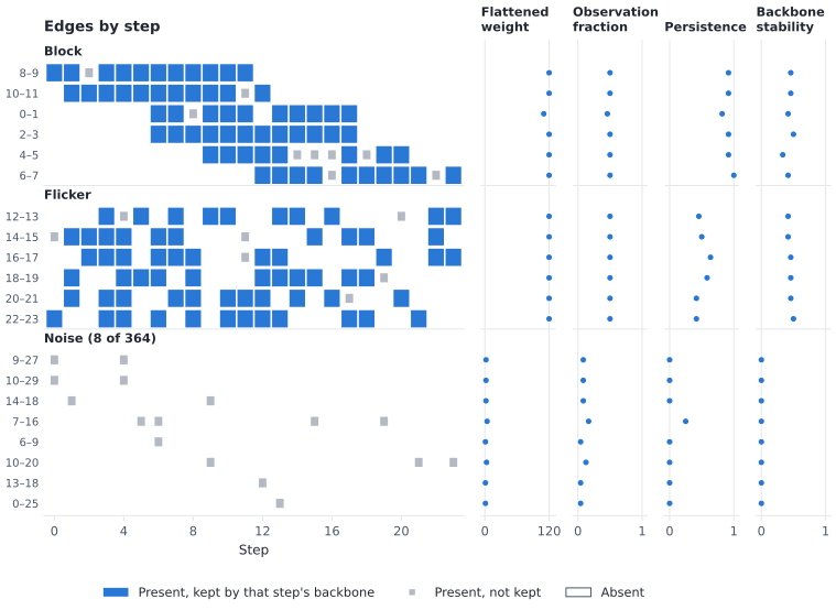
Edges by time. Block and flicker edges have the same flattened weight, observation fraction and stability; only persistence, which reads the order of the steps, tells them apart.

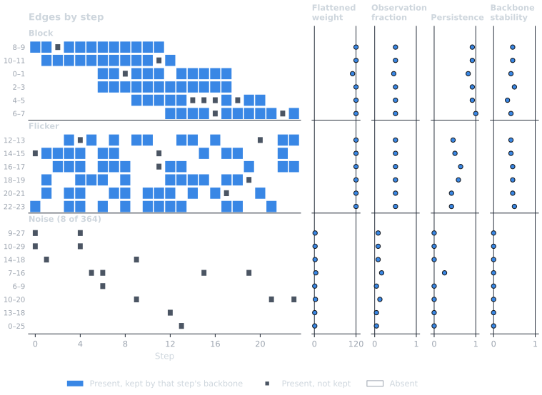
Edges by time. Block and flicker edges have the same flattened weight, observation fraction and stability; only persistence, which reads the order of the steps, tells them apart.

Two more things show in the grid. The per-step backbone keeps a heavy edge in some of its steps and drops it in others, because the disparity filter judges an edge against the other edges of its endpoints, which change from step to step; stability averages that churn out. And the block edge with a missed step has its run cut in two, so its persistence and longest run drop:

e, t_miss = DROPOUT
print(
    f"Edge {e[0]}–{e[1]} misses step {t_miss}: longest run "
    f"{pers.edges[e]['max_run']} steps, persistence {pers.edges[e]['persistence']:.2f}"
)

Edge 0–1 misses step 12: longest run 6 steps, persistence 0.82

A model of activity, below, treats such a gap differently.

Smoothing significance over time: the Kalman backbone

The scores so far count observations. They do not ask whether an edge’s weight is significant, and when weights are noisy, a single snapshot rarely says. Testing every snapshot separately and keeping the edges that pass in some step multiplies the false positives; flattening first loses the timing. kalman_backbone() sits between the two.

It runs a static significance test on every snapshot, turns each edge’s p-value into a probit score y = Φ⁻¹(1 − p) (a z-score: about 0 when nothing is going on, large when the edge is significant) and smooths each edge’s series of scores with a local-level model: the edge has an underlying level of significance that drifts slowly, and each step’s score is that level plus noise. The Kalman filter (Kalman, 1960) estimates the level from the steps up to each step; the Rauch-Tung-Striebel smoother (Rauch et al., 1965) also uses the later steps. half_life= sets how fast the level may drift: the weight of a step halves every half_life steps away. Because the smoothed level is a weighted sum of the scores, its distribution when no step carries a signal is known exactly, which gives a calibrated p-value per edge and step.

Note

The Kalman filter and smoother are standard; using them to smooth per-snapshot backbone significance is a novel adaptation proposed in this library’s design note (docs/design/temporal-backbones.md), not a published backbone method. For a fixed drift it amounts to a weighted Stouffer combination of the per-step evidence, localized in time. Read its results with the limits below in mind.

A rising block

The second synthetic network is a fixed stochastic block model: 30 nodes in three groups of 10, each pair linked with probability 0.3 inside a group and 0.05 across. The links stay the same in all 24 steps, but their weights are drawn afresh in every step, as counts with mean 3. Five planted edges inside the first group are rising: their mean weight is 3 up to step 11, and from step 12 on it grows by a fixed amount every step.

RISE, BASE, SLOPE = 12, 3.0, 0.6
rng = np.random.default_rng(11)
links = [
    (u, v)
    for u, v in combinations(range(30), 2)
    if rng.random() < (0.3 if u // 10 == v // 10 else 0.05)
]
rising = [(0, 1), (2, 3), (4, 5), (6, 7), (8, 9)]
links = sorted(set(links) | set(rising))
steady = [e for e in links if e not in rising]


def mean_weight(e, t):
    return BASE * (1 + SLOPE * max(0, t - RISE + 1)) if e in rising else BASE


sbm = {}
for t in range(N_STEPS):
    sbm[t] = nx.Graph()
    sbm[t].add_nodes_from(range(30))
    for e in links:
        sbm[t].add_edge(*e, weight=int(rng.geometric(1 / mean_weight(e, t))))
print(f"{len(links)} links: {len(rising)} rising, {len(steady)} steady")
print(
    f"Mean weight of a rising edge at the last step: {mean_weight(rising[0], N_STEPS - 1):.1f}"
)


def found(edges):
    """(rising edges among *edges*, other edges among *edges*)."""
    edges = {key(*e) for e in edges}
    return len(edges & set(rising)), len(edges - set(rising))

64 links: 5 rising, 59 steady
Mean weight of a rising edge at the last step: 24.6

The disparity filter, run on each snapshot, finds some rising edges once their weight has grown, but not reliably, and it keeps a few steady edges by chance in most steps:

raw = {t: nb.disparity_filter(G) for t, G in sbm.items()}
raw_found = {
    t: found(nb.threshold_filter(raw[t], "disparity_pvalue", ALPHA).edges) for t in sbm
}

Now the Kalman backbone on the same snapshots, with the same filter, a half-life of 3 steps, and both the smoother (all steps) and the filter (mode="filter", only the steps up to each one, as an online method would see them). kalman_snapshots() expands the per-step p-values into one graph per step, to be cut like any snapshot.

HALF_LIFE = 3
smoothed = nb.kalman_backbone(sbm, "disparity", half_life=HALF_LIFE, seed=0)
online = nb.kalman_backbone(
    sbm, "disparity", half_life=HALF_LIFE, mode="filter", seed=0
)
smooth_found, online_found = (
    {
        t: found(nb.threshold_filter(G, "kalman_pvalue", ALPHA).edges)
        for t, G in nb.kalman_snapshots(H).items()
    }
    for H in (smoothed, online)
)
SHOW = [
    RISE - 4,
    RISE - 2,
    RISE - 1,
    RISE,
    RISE + 1,
    RISE + 2,
    RISE + 4,
    RISE + 6,
    N_STEPS - 1,
]
print(
    f"Rising / other edges kept at p < {ALPHA}, by step (the rise starts at step {RISE}):"
)
table(
    ["Step", *map(str, SHOW)],
    [
        [name, *(f"{d[t][0]}/{d[t][1]}" for t in SHOW)]
        for name, d in (
            ("Per-step disparity", raw_found),
            ("Kalman smoother", smooth_found),
            ("Kalman filter", online_found),
        )
    ],
)

Rising / other edges kept at p < 0.05, by step (the rise starts at step 12):
Step                8    10   11   12   13   14   16   18   23
------------------  ---  ---  ---  ---  ---  ---  ---  ---  ---
Per-step disparity  0/0  0/1  0/0  0/2  2/3  3/1  3/1  4/2  4/3
Kalman smoother     1/0  2/0  3/0  3/0  5/0  5/0  5/0  5/0  5/0
Kalman filter       0/0  0/0  0/0  0/0  0/0  2/0  2/0  5/0  5/0

The figure shows every edge’s significance over time, as -log10(p): higher is more significant.

P_FLOOR = 1e-4


def series(H, attr, e):
    return [
        -math.log10(
            max(
                H[t].edges[e][attr] if isinstance(H, dict) else H.edges[e][attr][t],
                P_FLOOR,
            )
        )
        for t in range(N_STEPS)
    ]


def draw_kalman(mode):
    p = style.palette(mode)
    fig, axes = plt.subplots(1, 3, figsize=(9.6, 3.4), sharey=True)
    panels = [
        ("Per-step disparity filter", lambda e: series(raw, "disparity_pvalue", e)),
        (
            f"Kalman smoother (half-life {HALF_LIFE})",
            lambda e: series(smoothed, "kalman_pvalues", e),
        ),
        (
            "Kalman filter (past steps only)",
            lambda e: series(online, "kalman_pvalues", e),
        ),
    ]
    steps = list(range(N_STEPS))
    for ax, (title, get) in zip(axes, panels):
        ax.axvspan(RISE - 0.5, N_STEPS - 0.5, color=p.hairline, lw=0, zorder=0)
        for e in steady:
            ax.plot(steps, get(e), color=p.removed, lw=0.6, zorder=1)
        for e in rising:
            ax.plot(steps, get(e), color=p.kept, lw=1.5, zorder=2)
        ax.axhline(-math.log10(ALPHA), color=p.ink, lw=0.75, ls=(0, (3, 2)), zorder=3)
        ax.set_title(title, fontsize=9)
        ax.set_xlim(0, N_STEPS - 1)
        ax.set_xticks([0, 6, RISE, 18, N_STEPS - 1])
        ax.set_xlabel("Step")
    axes[0].set_ylabel("−log10(p)")
    axes[0].set_ylim(0, -math.log10(P_FLOOR) * 1.05)
    axes[0].text(
        RISE,
        -math.log10(P_FLOOR),
        " weights rise",
        va="top",
        ha="left",
        color=p.muted,
        fontsize=8,
    )
    fig.legend(
        handles=[
            Line2D([], [], color=p.kept, lw=1.5, label=f"Rising edges ({len(rising)})"),
            Line2D(
                [], [], color=p.removed, lw=1.5, label=f"Steady edges ({len(steady)})"
            ),
            Line2D([], [], color=p.ink, lw=0.75, ls=(0, (3, 2)), label="alpha = 0.05"),
            Patch(facecolor=p.hairline, label="Rising period"),
        ],
        loc="lower center",
        bbox_to_anchor=(0.5, -0.06),
        ncols=4,
    )
    fig.tight_layout(rect=(0, 0.08, 1, 1))
    return fig


save("temporal_kalman", draw_kalman)

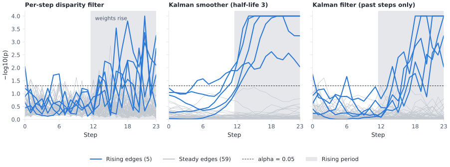
Per-step significance before and after smoothing, for the rising edges (blue) and the steady edges (gray). P-values below 1e-4 are drawn at the top.

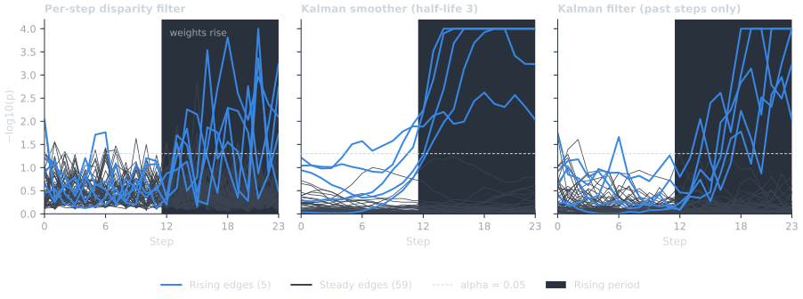
Per-step significance before and after smoothing, for the rising edges (blue) and the steady edges (gray). P-values below 1e-4 are drawn at the top.

Smoothing turns a jagged, noisy picture into a clear one: the steady edges sink, the rising ones climb and stay up. The filter, which may not look ahead, detects the rise later than the smoother.

The edge-level test

The per-step p-values are many tests, one per edge and step. Each edge also gets one edge-level p-value, kalman_pvalue, which tests its largest smoothed z-score over all steps against a simulated null. It is one test per edge, so a correction across edges (here Benjamini-Hochberg) is all it needs:

edge_bb = nb.threshold_filter(smoothed, "kalman_pvalue", ALPHA, mtc="bh")
n_rise, n_other = found(edge_bb.edges)
print(
    f"Edge-level backbone (BH at {ALPHA}): {n_rise} of {len(rising)} rising edges, "
    f"{n_other} of {len(steady)} steady edges"
)

Edge-level backbone (BH at 0.05): 4 of 5 rising edges, 0 of 59 steady edges

Which per-step test?

The smoother can only be as well calibrated as the test it smooths. Its p-values are exact when every step’s p-value is uniform under the null; any bias in the per-step test is added up over neighboring steps.

The disparity filter gives an edge the smaller of its two endpoints’ p-values. That minimum is pulled toward 0 even when nothing is going on, so kalman_backbone replaces each per-step p-value p by 1 − (1 − p)² by default (sidak=True, a Šidák correction). The two endpoint tests share the edge’s weight, so this overcorrects and the smoothed tests are conservative. One way to see the difference is to count, before the rise, how often the steady edges reach p < 0.05: a calibrated test does so in about 5% of edge-steps.

no_sidak = nb.kalman_backbone(
    sbm, "disparity", half_life=HALF_LIFE, sidak=False, seed=0
)


def null_rate(pvalue_at):
    hits = [pvalue_at(e, t) < ALPHA for e in steady for t in range(RISE)]
    return sum(hits) / len(hits)


rates = {
    "Per-step disparity": null_rate(lambda e, t: raw[t].edges[e]["disparity_pvalue"]),
    "Per-step disparity, Šidák-corrected": null_rate(
        lambda e, t: 1 - (1 - raw[t].edges[e]["disparity_pvalue"]) ** 2
    ),
    "Kalman smoother (sidak=True, default)": null_rate(
        lambda e, t: smoothed.edges[e]["kalman_pvalues"][t]
    ),
    "Kalman smoother (sidak=False)": null_rate(
        lambda e, t: no_sidak.edges[e]["kalman_pvalues"][t]
    ),
}
table(
    ["Steady edges, before the rise", "Share with p < 0.05"],
    [[name, f"{rate:.3f}"] for name, rate in rates.items()],
)

Steady edges, before the rise          Share with p < 0.05
-------------------------------------  -------------------
Per-step disparity                     0.025
Per-step disparity, Šidák-corrected    0.003
Kalman smoother (sidak=True, default)  0.000
Kalman smoother (sidak=False)          0.158

Without the correction, a small per-step bias becomes a large one after smoothing. With it, the test errs on the safe side: the smoothed backbone above keeps no steady edge in any step, at the cost of some power, which shows in how late the filter catches the rise. A test that judges each edge once, with continuous p-values, would avoid both problems. noise_corrected_filter() (Coscia & Neffke, 2017) judges each edge once, but its calibrated p-values are exact binomial tails, hence discrete; the p-value reading of the paper’s rule (pvalue_method="delta") is continuous but far too small on low-count snapshots (issue #105), so do not smooth it. Scorers with discrete p-values (the noise-corrected and marginal likelihood filters, ECM, LANS, Pólya and GloSS) need discrete="raw", which keeps the tests valid but conservative.

Limits and risks

Temporal leakage. The smoothed p-values are exact for the null of no signal at any step, not for “no signal at this step”. A signal in some steps raises the smoothed level of nearby steps too, so the smoother can flag an edge before its weight changed. The filter only looks back, so it cannot flag an edge early, but it is late:

early = {
    name: sum(d[t][0] for t in range(RISE - HALF_LIFE, RISE))
    for name, d in (
        ("Per-step disparity", raw_found),
        ("Kalman smoother", smooth_found),
        ("Kalman filter", online_found),
    )
}
print(f"Rising edges flagged in the {HALF_LIFE} steps before the rise:")
table(["Method", "Edge-steps flagged"], [[k, v] for k, v in early.items()])

Rising edges flagged in the 3 steps before the rise:
Method              Edge-steps flagged
------------------  ------------------
Per-step disparity  0
Kalman smoother     6
Kalman filter       0

So read a smoothed backbone at step t as “this edge is significant around step t”, not “at step t”, and use mode="filter" when the timing of an onset matters. Two further cautions (see the Notes of kalman_backbone()):

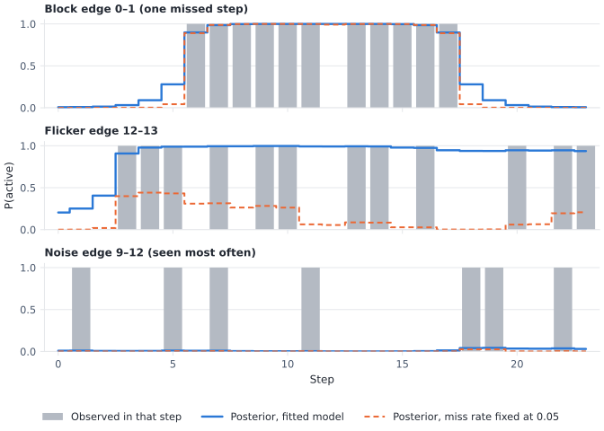
• Persistent confounders. Anything that makes a pair’s scores correlated over time under the null, such as a stable dyad-level effect that the static test does not model, makes the tests anti-conservative. Check that each edge’s kalman_innovations, its standardized one-step prediction errors, look like white noise.

• Many tests. The per-step p-values are E × T tests. Correct them within each step (for example with kalman_snapshots() and threshold_filter(..., mtc="bh")), or use the edge-level kalman_pvalue.

Persistent activity: a hidden Markov model

Back to the first network. Persistence takes every observation at face value: one missed step cuts a run in two, and one stray observation starts a run. edge_persistence_hmm() instead treats each edge as switching between two hidden states, inactive and active, as a Markov chain, and treats what is seen as a noisy flag of the state: an active edge can be missed (at rate beta) and an inactive one seen (at rate alpha). One set of these rates, shared by all edges, is fitted by expectation-maximization. Each edge gets hmm_posterior, its posterior probability of being active in each step given all of its observations. The model is a standard two-state hidden Markov model; using it for temporal backbones is proposed in the design note.

hmm = nb.edge_persistence_hmm(snaps)
fit = hmm.graph["temporal"]["hmm"]
print(
    "Fitted: "
    + ", ".join(f"{k} = {fit[k]:.3f}" for k in ("a01", "a10", "alpha", "beta"))
)
table(
    ["hmm_n_active (group mean)", *GROUPS],
    [
        [
            "Fitted model",
            *(f"{group_mean(hmm, 'hmm_n_active', e):.1f}" for e in GROUPS.values()),
        ]
    ],
)

Fitted: a01 = 0.002, a10 = 0.071, alpha = 0.092, beta = 0.299
hmm_n_active (group mean)  Block  Flicker  Noise
-------------------------  -----  -------  -----
Fitted model               12.2   18.3     0.0

The fit reads the noise as the inactive state, seen now and then (alpha), and it fills the block edge’s missed step:

e, t_miss = DROPOUT
print(
    f"Posterior that {e[0]}–{e[1]} is active in its missed step {t_miss}: "
    f"{hmm.edges[e]['hmm_posterior'][t_miss]:.3f}"
)

Posterior that 0–1 is active in its missed step 12: 0.999

But it reads the flicker edges as active. One set of parameters is shared by every edge, so a gap in an edge’s record has two explanations: the edge switched off (the switching rate a10) or it stayed active and was missed (the miss rate beta). No single chain fits both a block that stays on and flicker that comes and goes at random, and on these data the likelihood prefers a large miss rate with slow switching. An edge seen in half of the steps all the way through then looks like one long active spell that was often missed, so the flicker edges get more active steps than the block. This is the best fit, not a bad start: more EM starts (n_init=) find the same one.

What counts as “active” is a modeling choice. If an active tie should be seen in nearly every step, say so: fixing the miss rate with params= makes the model read the gaps as inactivity instead.

BETA = 0.05
hmm_fixed = nb.edge_persistence_hmm(snaps, params={"beta": BETA})
table(
    ["hmm_n_active (group mean)", *GROUPS],
    [
        [name, *(f"{group_mean(H, 'hmm_n_active', e):.1f}" for e in GROUPS.values())]
        for name, H in (
            ("Fitted model", hmm),
            (f"Miss rate fixed at {BETA}", hmm_fixed),
        )
    ],
)

hmm_n_active (group mean)  Block  Flicker  Noise
-------------------------  -----  -------  -----
Fitted model               12.2   18.3     0.0
Miss rate fixed at 0.05    12.0   7.2      0.0

You can spot this case without knowing the truth. Next to the fitted parameters, H.graph["temporal"]["hmm"] records n_active_steps, the number of steps the most likely paths mark active, and unobserved_active_share, the share of them in which the edge was not seen. A large share means that much of the “activity” is inferred rather than observed:

fit_fixed = hmm_fixed.graph["temporal"]["hmm"]
table(
    ["Model", "beta", "a10", "Active steps", "Share not observed"],
    [
        [
            name,
            f"{m['beta']:.2f}",
            f"{m['a10']:.3f}",
            f"{m['n_active_steps']}",
            f"{m['unobserved_active_share']:.2f}",
        ]
        for name, m in (
            ("Fitted model", fit),
            (f"Miss rate fixed at {BETA}", fit_fixed),
        )
    ],
)

Model                    beta  a10    Active steps  Share not observed
-----------------------  ----  -----  ------------  ------------------
Fitted model             0.30  0.071  183           0.26
Miss rate fixed at 0.05  0.05  0.133  115           0.08

The data alone cannot always tell this case from a measurement process that really does miss that many active steps, so the function does not warn: it records the numbers and leaves the call to you. When the share is large, compare hmm_n_active with the observation fraction and the longest run, and fix beta if you know how the ties were recorded. Fixing it is not a cure-all: the switching rates are still shared, and when nearly every edge in the fit is persistent they come out so slow that a flickering edge can still read as active.

The figure compares the raw presence of three edges with both models’ posteriors: the block edge with the missed step, a flicker edge, and the noise edge seen most often.

noisiest = max(noise, key=lambda e: (flat.edges[e]["n_obs"], e))
EXAMPLES = [
    (f"Block edge {DROPOUT[0][0]}–{DROPOUT[0][1]} (one missed step)", DROPOUT[0]),
    (f"Flicker edge {flicker[0][0]}–{flicker[0][1]}", flicker[0]),
    (f"Noise edge {noisiest[0]}–{noisiest[1]} (seen most often)", noisiest),
]


def draw_hmm(mode):
    p = style.palette(mode)
    c_fit, c_fixed = style.categorical(2, mode)
    fig, axes = plt.subplots(3, 1, figsize=(7.2, 5.0), sharex=True)
    steps = list(range(N_STEPS))
    for ax, (title, e) in zip(axes, EXAMPLES):
        seen = [t for t in steps if snaps[t].has_edge(*e)]
        ax.bar(
            seen,
            [1] * len(seen),
            width=0.8,
            color=p.node_removed,
            linewidth=0,
            zorder=1,
        )
        fitted = [hmm.edges[e]["hmm_posterior"][t] for t in steps]
        fixed = [hmm_fixed.edges[e]["hmm_posterior"][t] for t in steps]
        ax.plot(steps, fitted, color=c_fit, lw=1.8, drawstyle="steps-mid", zorder=3)
        ax.plot(
            steps,
            fixed,
            color=c_fixed,
            lw=1.5,
            ls=(0, (3, 2)),
            drawstyle="steps-mid",
            zorder=4,
        )
        ax.set_ylim(0, 1.05)
        ax.set_yticks([0, 0.5, 1])
        ax.set_title(title, fontsize=9)
        ax.grid(True, axis="y")
    axes[1].set_ylabel("P(active)")
    axes[-1].set_xlabel("Step")
    axes[-1].set_xlim(-0.6, N_STEPS - 0.4)
    fig.legend(
        handles=[
            Patch(facecolor=p.node_removed, label="Observed in that step"),
            Line2D([], [], color=c_fit, lw=1.8, label="Posterior, fitted model"),
            Line2D(
                [],
                [],
                color=c_fixed,
                lw=1.5,
                ls=(0, (3, 2)),
                label=f"Posterior, miss rate fixed at {BETA}",
            ),
        ],
        loc="lower center",
        bbox_to_anchor=(0.5, -0.02),
        ncols=3,
    )
    fig.tight_layout(rect=(0, 0.06, 1, 1))
    return fig


save("temporal_hmm", draw_hmm)

Raw presence (gray bars) against the posterior probability of being active, for the fitted model (solid) and with the miss rate fixed (dashed).

Raw presence (gray bars) against the posterior probability of being active, for the fitted model (solid) and with the miss rate fixed (dashed).

hmm_score (an edge’s largest posterior) and hmm_active_fraction (its mean posterior) are membership scores, not p-values: they are probabilities under a model fitted to the same data, which assumes that every edge follows one shared chain. Cut them with threshold_filter(), or use hmm_keep (min_steps=), but do not read the cut as a significance level.

Choosing among them

Each method answers a different question, so the right one depends on what “important over time” means for your data. To make that concrete, score both synthetic networks with every method and take as many top-scored edges as there are planted ones (the block in the first network, the rising edges in the second). The table gives the share of planted edges among them: 1 means the score ranks every planted edge first. Ties are split evenly, so a score that cannot tell edges apart gets the share of planted edges among the tied ones.

def top_share(scores, targets):
    """Expected share of *targets* among the top len(targets) scores."""
    k = len(targets)
    values = {e: (-math.inf if math.isnan(s) else s) for e, s in scores.items()}
    cut = sorted(values.values(), reverse=True)[k - 1]
    above = [e for e, s in values.items() if s > cut]
    tied = [e for e, s in values.items() if s == cut]
    hits = sum(e in targets for e in above)
    hits += (k - len(above)) * sum(e in targets for e in tied) / len(tied)
    return hits / k


def scores_of(H, attr):
    return {key(u, v): d[attr] for u, v, d in H.edges(data=True)}


def all_scores(T):
    """Every method's edge score on the snapshots *T*."""
    with warnings.catch_warnings():
        # In the second network every link is present in every step, so the
        # HMM's two states cannot be told apart and its fit warns.
        warnings.simplefilter("ignore", RuntimeWarning)
        hmm_fit = nb.edge_persistence_hmm(T)
        hmm_beta = nb.edge_persistence_hmm(T, params={"beta": BETA})
    return {
        "Flattened weight": scores_of(nb.flatten_temporal(T), "weight"),
        "Observation fraction": scores_of(nb.observation_fraction(T), "obs_fraction"),
        "Persistence (longest run)": scores_of(nb.persistence(T), "max_run"),
        "Backbone stability": scores_of(
            nb.backbone_stability(T, nb.disparity_filter, threshold=ALPHA), "stability"
        ),
        "Weight trend (slope)": scores_of(nb.weight_trend(T), "weight_slope"),
        "HMM, fitted (mean posterior)": scores_of(hmm_fit, "hmm_active_fraction"),
        f"HMM, beta = {BETA} (mean posterior)": scores_of(
            hmm_beta, "hmm_active_fraction"
        ),
        "Kalman (edge z-score)": scores_of(
            nb.kalman_backbone(T, "disparity", half_life=HALF_LIFE, seed=0),
            "kalman_score",
        ),
    }


compare = {"block": all_scores(snaps), "rising": all_scores(sbm)}
share = {
    (name, target): top_share(compare[target][name], set(edges))
    for target, edges in (("block", block), ("rising", rising))
    for name in compare[target]
}
table(
    ["Method", "Block (network 1)", "Rising (network 2)"],
    [
        [name, f"{share[name, 'block']:.2f}", f"{share[name, 'rising']:.2f}"]
        for name in compare["block"]
    ],
)

Method                             Block (network 1)  Rising (network 2)
---------------------------------  -----------------  ------------------
Flattened weight                   0.45               1.00
Observation fraction               0.45               0.08
Persistence (longest run)          1.00               0.08
Backbone stability                 0.43               1.00
Weight trend (slope)               0.33               1.00
HMM, fitted (mean posterior)       0.00               0.08
HMM, beta = 0.05 (mean posterior)  1.00               0.08
Kalman (edge z-score)              0.83               1.00

Reading the table:

• On the first network, the scores that count steps (flattened weight, observation fraction, stability) cannot separate the block from the flicker. The longest run, which reads the order of the steps, can. The fitted HMM prefers the flicker, as we saw, until its miss rate is fixed. The Kalman backbone also favors the block: absent steps count as observed zeros, and significance in consecutive steps adds up where scattered significance does not.

• On the second network every link is present in every step, so the presence-based scores tie and do no better than chance, while the scores that read the weights find the rise (stability reads them through the per-step backbones). The weight trend finds it because this rise is a straight line; it is a description, not a test. The flattened weight finds the rising edges because they end up heavier in total, but it cannot say when.

The table summarizes two toy networks; it is not a benchmark. What it shows is that each score sees one kind of structure.

Method	Question it answers	Output	Use it when
flatten_temporal(), then a static method	Which pairs are important overall?	A static graph; any static backbone	Timing does not matter, or the network is one aggregate by design.
observation_fraction()	How often is the edge seen?	A share of eligible steps	Frequency of contact is the point; a quick first filter.
persistence()	Does the edge stay on once it appears?	Run lengths and a “stays on” share	You want lasting ties rather than frequent but scattered ones.
backbone_stability()	How often does a static backbone keep the edge?	A share of eligible steps	You trust a static method per step and want a consensus over time.
weight_trend()	Is the edge’s weight growing, fading or erratic?	Mean, spread, coefficient of variation, slope	Describing change; it is not a test.
edge_persistence_hmm()	Is the edge in a persistently active state, allowing for missed and stray observations?	Posterior probabilities (membership scores, not p-values)	Observations are noisy and you can say what an active tie looks like (fix params= if the fit’s idea differs from yours).
kalman_backbone()	Is the edge’s weight significant around each step, pooling neighboring steps?	Per-step and edge-level p-values	Weights are noisy and you need a test; mind leakage, use a calibrated per-step test, and correct for multiple tests.

A short decision guide:

1. Decide what a step is (the bin width) and what a weight means before anything else; both change every score.

2. If only “overall” matters, flatten and use a static method.

3. If presence is what you have, start with the observation fraction and persistence; move to the HMM when single missed or stray observations should not count.

4. If weights carry the signal and you need significance, use kalman_backbone with the edge-level kalman_pvalue, corrected across edges, and mode="filter" when onsets must not leak backward.

5. Report the bin width, the method and its settings (half_life, fixed HMM parameters, the per-step test and cut) with the backbone; describe_backbone() writes that paragraph from the scored graph’s graph["temporal"] record.

Where next

• API: Temporal (every function’s parameters, Notes and examples) and Filters for threshold_filter() and boolean_filter().

• User guide: Temporal networks: formats and conversions (the three forms and every conversion) and Temporal backbones: presence and eligible steps (how absent edges and absent nodes are counted).

• Tutorials: Temporal Backbones (the calls, score by score), Statistical null models side by side (the static tests the Kalman backbone smooths) and Validating a Backbone (multiple testing).

References

• Coscia, M., & Neffke, F. M. (2017). Network backboning with noisy data. Proceedings of the IEEE International Conference on Data Engineering (ICDE), 425-436. https://doi.org/10.1109/ICDE.2017.100

• Kalman, R. E. (1960). A new approach to linear filtering and prediction problems. Journal of Basic Engineering, 82(1), 35-45. https://doi.org/10.1115/1.3662552

• Rauch, H. E., Tung, F., & Striebel, C. T. (1965). Maximum likelihood estimates of linear dynamic systems. AIAA Journal, 3(8), 1445-1450. https://doi.org/10.2514/3.3166

• Serrano, M. A., Boguñá, M., & Vespignani, A. (2009). Extracting the multiscale backbone of complex weighted networks. Proceedings of the National Academy of Sciences, 106(16), 6483-6488. https://doi.org/10.1073/pnas.0808904106