Bipartite Methods#
Examples in this module use nx.davis_southern_women_graph().
Projection scoring methods return full graphs with p-values/weights; use
threshold_filter() or
boolean_filter() as needed, or
backbone_from_projection(), which keeps only the
significant pairs.
Complexity classes are provided in each function docstring.
Every function accepts either a bipartite graph with its agent_nodes or an
agents x artifacts incidence matrix (NumPy array, SciPy sparse array or matrix,
or pandas DataFrame) with optional agent_labels / artifact_labels.
The incidence is kept sparse and agent pairs are scored in blocks of rows.
The simple, hyperbolic, ProbS and YCN weightings follow Coscia & Rossi (2019,
doi:10.1145/3341161.3342862,
arXiv:1906.09081). The hyperbolic weight uses 1/d(z) per shared artifact;
hyper_projection(..., newman=True) (method="newman") gives Newman’s
(2001) 1/(d(z) - 1) collaboration weight.
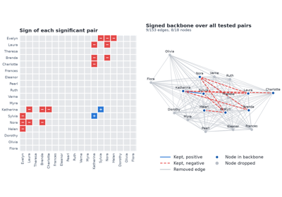
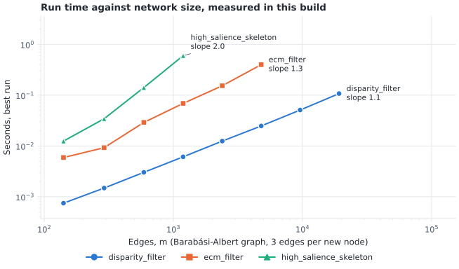
For a narrative walkthrough with figures (projection weights, the null models side by side, the FDSM p-value floor, signed backbones, SDSM-EC, matching R and sparse input), see Bipartite projections and their backbones.
Bipartite projection backbone methods.
These methods operate on bipartite networks and extract significant edges in the one-mode projection among “agent” nodes.
Every function accepts either an undirected bipartite NetworkX graph B
with its agent nodes, or an agents x artifacts incidence matrix (a NumPy
array, a SciPy sparse array or matrix, or a pandas DataFrame) with
optional agent_labels / artifact_labels, as R backbone does.
Internally the incidence is kept as a SciPy CSR sparse array and agent
co-occurrences are computed with sparse products, one block of agent rows at
a time, so no dense agents x agents matrix is ever formed.
Methods#
- simple_projection
Shared-neighbor (co-occurrence count) projection.
- hyper_projection
Hyperbolic projection,
1 / d(z)per shared artifact (or Newman’s1 / (d(z) - 1)withnewman=True).- probs_projection
ProbS (mass-diffusion) random-walk projection.
- ycn_projection
YCN stationary random-walk flow projection.
- sdsm
Stochastic Degree Sequence Model (Neal 2014).
- fdsm
Fixed Degree Sequence Model (Neal et al. 2021).
- fixedfill, fixedrow, fixedcol
Fixed fill / row / column null models (Neal et al. 2021).
- nx_backbone.simple_projection(B, agent_nodes=None, weight='weight', *, agent_labels=None, artifact_labels=None)[source]#
Project a bipartite graph using shared-neighbor counts.
The weight of agents
uandvis the number of artifacts they share [1]:\[w_{uv} = |\Gamma(u) \cap \Gamma(v)|\]This equals
weighted_projected_graph().- Parameters:
- Bgraph or array-like
An undirected bipartite NetworkX graph, or an agents x artifacts binary incidence matrix (NumPy array, SciPy sparse array or matrix, or pandas
DataFrame).- agent_nodesiterable or None, optional (default=None)
Nodes in the “agent” partition of a graph B (one full side of the bipartition). If
Nonethey are inferred as inbackbone_from_projection(). Must beNonefor a matrix B.- weightstring, optional (default=”weight”)
Edge attribute name for the projection weight.
- agent_labels, artifact_labelssequence or None, optional
Row and column labels of a matrix B (default
0, 1, ..., or aDataFrame’s index and columns). Only valid with a matrix B.
- Returns:
- projectiongraph
Undirected graph on the agent nodes; pairs with a positive weight are joined by an edge carrying the weight attribute.
- Raises:
- NetworkXError
If B is not bipartite or agent_nodes is not one side of it.
- NetworkXNotImplemented
If B is directed or a multigraph.
- ValueError
If a matrix B is not two-dimensional and binary, or its labels do not match its shape.
References
[1]Coscia, M. & Rossi, L. (2019). The impact of projection and backboning on network topologies. Proc. IEEE/ACM ASONAM 2019. https://doi.org/10.1145/3341161.3342862 (arXiv:1906.09081).
Examples
>>> import networkx as nx
>>> from nx_backbone import simple_projection
>>> B = nx.Graph([(1, "a"), (1, "b"), (2, "a"), (2, "c"), (3, "b"), (3, "c")])
>>> P = simple_projection(B, agent_nodes=[1, 2, 3])
>>> sorted(P.edges(data="weight"))
[(1, 2, 1.0), (1, 3, 1.0), (2, 3, 1.0)]
An agents x artifacts incidence matrix works directly:
>>> import numpy as np
>>> M = np.array([[1, 1, 0], [1, 0, 1], [0, 1, 1]])
>>> P = simple_projection(M, agent_labels=[1, 2, 3])
>>> sorted(P.edges(data="weight"))
[(1, 2, 1.0), (1, 3, 1.0), (2, 3, 1.0)]
Computational complexity estimate is
O(e_b + n_a^2 + sum_z d(z)^2)time andO(e_b + B)space.
- nx_backbone.hyper_projection(B, agent_nodes=None, weight='weight', *, newman=False, agent_labels=None, artifact_labels=None)[source]#
Project a bipartite graph with hyperbolic (degree-discounted) weights.
Each shared artifact
zcontributes the inverse of its degreed(z) = |\Gamma(z)|, so sharing a small artifact counts for more than sharing a large one:\[w_{uv} = \sum_{z \in \Gamma(u) \cap \Gamma(v)} \frac{1}{d(z)}\]This is the “hyperbolic” projection as defined by Coscia & Rossi [1], who attribute the idea to Newman [2]. Newman’s own collaboration weight [3] discounts by
d(z) - 1instead, the number of other co-authors, so that each author’s ties sum to the number of their multi-author papers:\[w_{uv} = \sum_{z \in \Gamma(u) \cap \Gamma(v)} \frac{1}{d(z) - 1}\]Pass
newman=Truefor that variant; it equalscollaboration_weighted_projected_graph(). The two weightings coincide only up to a constant when every artifact has the same degree, so they can rank pairs differently.- Parameters:
- Bgraph or array-like
An undirected bipartite NetworkX graph, or an agents x artifacts binary incidence matrix (NumPy array, SciPy sparse array or matrix, or pandas
DataFrame).- agent_nodesiterable or None, optional (default=None)
Nodes in the “agent” partition of a graph B. If
Nonethey are inferred as inbackbone_from_projection(). Must beNonefor a matrix B.- weightstring, optional (default=”weight”)
Edge attribute name for the projection weight.
- newmanbool, optional (default=False)
If
Trueuse Newman’s1 / (d(z) - 1)discount.- agent_labels, artifact_labelssequence or None, optional
Row and column labels of a matrix B. Only valid with a matrix B.
- Returns:
- projectiongraph
Undirected weighted graph on the agent nodes.
- Raises:
- NetworkXError
If B is not bipartite or agent_nodes is not one side of it.
- NetworkXNotImplemented
If B is directed or a multigraph.
- ValueError
If a matrix B is not two-dimensional and binary, or its labels do not match its shape.
See also
References
[1]Coscia, M. & Rossi, L. (2019). The impact of projection and backboning on network topologies. Proc. IEEE/ACM ASONAM 2019. https://doi.org/10.1145/3341161.3342862 (arXiv:1906.09081).
[2]Newman, M. E. J. (2001). Scientific collaboration networks. I. Network construction and fundamental results. Physical Review E, 64, 016131.
[3]Newman, M. E. J. (2001). Scientific collaboration networks. II. Shortest paths, weighted networks, and centrality. Physical Review E, 64, 016132.
Examples
>>> import networkx as nx
>>> from nx_backbone import hyper_projection
>>> B = nx.Graph([(1, "a"), (1, "b"), (2, "a"), (2, "c"), (3, "b"), (3, "c")])
>>> P = hyper_projection(B, agent_nodes=[1, 2, 3])
>>> sorted(P.edges(data="weight"))
[(1, 2, 0.5), (1, 3, 0.5), (2, 3, 0.5)]
>>> P = hyper_projection(B, agent_nodes=[1, 2, 3], newman=True)
>>> sorted(P.edges(data="weight"))
[(1, 2, 1.0), (1, 3, 1.0), (2, 3, 1.0)]
Computational complexity estimate is
O(e_b + n_a^2 + sum_z d(z)^2)time andO(e_b + B)space.
- nx_backbone.probs_projection(B, agent_nodes=None, weight='weight', directed=False, *, agent_labels=None, artifact_labels=None)[source]#
Project a bipartite graph using ProbS random-walk weights.
ProbS (probabilistic spreading, or mass diffusion) [1] [2] sends a unit of resource from agent
uevenly to its artifacts, and from each artifact evenly to that artifact’s agents. The share ofu’s resource that reachesvis the directed weight\[w_{u \to v} = \frac{1}{d(u)} \sum_{z \in \Gamma(u) \cap \Gamma(v)} \frac{1}{d(z)},\]the probability that a two-step random walk from
uends atv. Zhou et al. [2] write the same matrix with the indices swapped (w_{vu}). As in Coscia & Rossi [1], the undirected projection averages the two directions,(w_{u \to v} + w_{v \to u}) / 2.- Parameters:
- Bgraph or array-like
An undirected bipartite NetworkX graph, or an agents x artifacts binary incidence matrix (NumPy array, SciPy sparse array or matrix, or pandas
DataFrame).- agent_nodesiterable or None, optional (default=None)
Nodes in the “agent” partition of a graph B. If
Nonethey are inferred as inbackbone_from_projection(). Must beNonefor a matrix B.- weightstring, optional (default=”weight”)
Edge attribute name for the projection weight.
- directedbool, optional (default=False)
If
Truereturn the asymmetric scores as aDiGraph; otherwise the two directions are averaged.- agent_labels, artifact_labelssequence or None, optional
Row and column labels of a matrix B. Only valid with a matrix B.
- Returns:
- Raises:
- NetworkXError
If B is not bipartite or agent_nodes is not one side of it.
- NetworkXNotImplemented
If B is directed or a multigraph.
- ValueError
If a matrix B is not two-dimensional and binary, or its labels do not match its shape.
See also
References
[1] (1,2)Coscia, M. & Rossi, L. (2019). The impact of projection and backboning on network topologies. Proc. IEEE/ACM ASONAM 2019. https://doi.org/10.1145/3341161.3342862 (arXiv:1906.09081).
Examples
>>> import networkx as nx
>>> from nx_backbone import probs_projection
>>> B = nx.Graph([("a", "x"), ("a", "y"), ("b", "x"), ("c", "y")])
>>> P = probs_projection(B, agent_nodes=["a", "b", "c"], directed=True)
>>> P["a"]["b"]["weight"], P["b"]["a"]["weight"]
(0.25, 0.5)
Computational complexity estimate is
O(e_b + n_a^2 + sum_z d(z)^2)time andO(e_b + B)space.
- nx_backbone.ycn_projection(B, agent_nodes=None, weight='weight', directed=False, max_iter=1000, tol=1e-12, *, agent_labels=None, artifact_labels=None)[source]#
Project a bipartite graph using YCN random-walk stationary flow.
YCN (Yildirim & Coscia [1], who call it BPR) extends ProbS to random walks of unbounded length. With the ProbS transition matrix
T_{uv} = w_{u \to v}(including the walk’s return tou) and its stationary distributionpi, reached by power iteration from the uniform vector, the directed weight is the stationary flow\[U_{uv} = \pi_u T_{uv}.\]The undirected projection averages
U_{uv}andU_{vu}[2]. On a connected bipartite graphpi_u = d(u) / |E|, so YCN equals the hyperbolic weight divided by the number of bipartite edges|E|and is already symmetric. On a disconnected graph the walk keeps each component’s initial mass,pi_u = (n_c / n) d(u) / |E_c|for a component withn_cof thenagents and|E_c|edges. Agents without artifacts get no edges.- Parameters:
- Bgraph or array-like
An undirected bipartite NetworkX graph, or an agents x artifacts binary incidence matrix (NumPy array, SciPy sparse array or matrix, or pandas
DataFrame).- agent_nodesiterable or None, optional (default=None)
Nodes in the “agent” partition of a graph B. If
Nonethey are inferred as inbackbone_from_projection(). Must beNonefor a matrix B.- weightstring, optional (default=”weight”)
Edge attribute name for the projection weight.
- directedbool, optional (default=False)
If
Truereturn the asymmetric flows as aDiGraph; otherwise the two directions are averaged.- max_iterint, optional (default=1000)
Maximum power iterations for the stationary distribution.
- tolfloat, optional (default=1e-12)
L1 convergence tolerance for the stationary distribution.
- agent_labels, artifact_labelssequence or None, optional
Row and column labels of a matrix B. Only valid with a matrix B.
- Returns:
- Raises:
- NetworkXError
If B is not bipartite or agent_nodes is not one side of it.
- NetworkXNotImplemented
If B is directed or a multigraph.
- ValueError
If a matrix B is not two-dimensional and binary, or its labels do not match its shape.
See also
References
[1]Yildirim, M. A., & Coscia, M. (2014). Using random walks to generate associations between objects. PLoS ONE, 9(8), e104813.
[2]Coscia, M. & Rossi, L. (2019). The impact of projection and backboning on network topologies. Proc. IEEE/ACM ASONAM 2019. https://doi.org/10.1145/3341161.3342862 (arXiv:1906.09081).
Examples
>>> import networkx as nx
>>> from nx_backbone import ycn_projection
>>> B = nx.Graph([(1, "a"), (1, "b"), (2, "a"), (2, "c"), (3, "b"), (3, "c")])
>>> P = ycn_projection(B, agent_nodes=[1, 2, 3])
>>> round(P[1][2]["weight"], 4)  # hyperbolic weight 0.5 / 6 edges
0.0833
Computational complexity estimate is
O(I e_b + n_a^2 + sum_z d(z)^2)time andO(e_b + B)space.
- nx_backbone.bipartite_projection(B, agent_nodes=None, method='simple', weight='weight', directed=False, max_iter=1000, tol=1e-12, *, agent_labels=None, artifact_labels=None)[source]#
Dispatch weighted bipartite projections by method name.
- Parameters:
- Bgraph or array-like
An undirected bipartite NetworkX graph, or an agents x artifacts binary incidence matrix (NumPy array, SciPy sparse array or matrix, or pandas
DataFrame).- agent_nodesiterable or None, optional (default=None)
Nodes in the “agent” partition of a graph B. If
Nonethey are inferred as inbackbone_from_projection(). Must beNonefor a matrix B.- method{“simple”, “hyper”, “newman”, “probs”, “ycn”}, optional
Projection weighting (default
"simple"): seesimple_projection(),hyper_projection()("hyper", alias"hyperbolic";"newman", alias"collaboration", ishyper_projection(..., newman=True)),probs_projection()andycn_projection().- weightstring, optional (default=”weight”)
Edge attribute name for the projection weight.
- directedbool, optional (default=False)
Return directed scores; only supported for
"probs"and"ycn".- max_iterint, optional (default=1000)
Maximum iterations for
method="ycn".- tolfloat, optional (default=1e-12)
Convergence tolerance for
method="ycn".- agent_labels, artifact_labelssequence or None, optional
Row and column labels of a matrix B. Only valid with a matrix B.
- Returns:
- projectiongraph
Weighted projection on the agent nodes.
- Raises:
- ValueError
If method is unknown,
directed=Trueis requested for a symmetric method, or a matrix B is invalid.- NetworkXError
If B is not bipartite or agent_nodes is not one side of it.
- NetworkXNotImplemented
If B is directed or a multigraph.
Examples
>>> import networkx as nx
>>> from nx_backbone import bipartite_projection
>>> B = nx.davis_southern_women_graph()
>>> women = [n for n, d in B.nodes(data=True) if d["bipartite"] == 0]
>>> P = bipartite_projection(B, women, method="hyper")
>>> P.number_of_nodes()
18
Computational complexity estimate is
O(I e_b + n_a^2 + sum_z d(z)^2)time andO(e_b + B)space.
- nx_backbone.sdsm(B, agent_nodes=None, alpha=0.05, weight=None, signed=False, prohibited=None, required=None, projection='simple', projection_weight='weight', projection_directed=False, projection_max_iter=1000, projection_tol=1e-12, pvalue_method='auto', *, agent_labels=None, artifact_labels=None)[source]#
Score a bipartite projection using the SDSM.
The Stochastic Degree Sequence Model [1] treats each bipartite edge as an independent Bernoulli variable whose probability
P[i, k]comes from the Bipartite Configuration Model (BiCM, seebicm()), the maximum-entropy model whose expected row and column sums equal the observed agent and artifact degrees. The co-occurrence count of agentsiandjis then a Poisson-binomial variable with success probabilitiesP[i, k] * P[j, k], and the p-value is its upper tail at the observed count. By default the tail is computed exactly, by convolution; Rbackboneevaluates it with the refined normal approximation (RNA) of Hong (2013) [3], which is available withpvalue_method="rna"(see Notes).Without edge constraints the BiCM probabilities depend only on the agent and artifact degrees, so the tails are computed once per pair of distinct agent degrees and the incidence matrix stays sparse.
- Parameters:
- Bgraph or array-like
An undirected bipartite NetworkX graph, or an agents x artifacts binary incidence matrix (NumPy array, SciPy sparse array or matrix, or pandas
DataFrame).- agent_nodesiterable or None, optional (default=None)
Nodes in the “agent” partition of a graph B. If
Nonethey are inferred as inbackbone_from_projection(). Must beNonefor a matrix B.- alphafloat, optional (default=0.05)
Retained for API compatibility. This function returns the full projected graph with p-values on all edges; apply
threshold_filter()(or usebackbone_from_projection()) to select significant edges.- weightNone or string, optional (default=None)
Not used for SDSM (bipartite is unweighted); reserved for API consistency.
- signedbool, optional (default=False)
If
True, run a two-tailed test: the stored p-value becomes two-sided and a"sign"edge attribute marks significantly strong (+1) versus significantly weak (-1) co-occurrences.- prohibitediterable of (agent, artifact) pairs or None, optional
SDSM-EC edge constraints (Neal & Neal, 2023) [2]: cells fixed to probability 0 in the null model (edges that cannot occur). Pairs that are edges of B contradict the data and are ignored with a
RuntimeWarning.- requirediterable of (agent, artifact) pairs or None, optional
SDSM-EC edge constraints: cells fixed to probability 1 in the null model (edges that must occur). Pairs that are not edges of B contradict the data and are ignored with a
RuntimeWarning. With constraints the BiCM is refitted on the unconstrained cells only, so expected degrees still match the observed ones. Constraints use a densen_agents x n_artifactsprobability matrix. If no constraint remains (none given, or all ignored), the result equals the unconstrained SDSM.- projection{“simple”, “hyper”, “newman”, “probs”, “ycn”}, optional
Projection weighting assigned to each returned edge (see
bipartite_projection()).- projection_weightstr, optional (default=”weight”)
Edge attribute name for the projection weight.
- projection_directedbool, optional (default=False)
Whether to use directed projection scores. Not supported for the undirected backbone output.
- projection_max_iterint, optional (default=1000)
Maximum iterations for
projection="ycn".- projection_tolfloat, optional (default=1e-12)
Convergence tolerance for
projection="ycn".- pvalue_method{“auto”, “exact”, “rna”}, optional (default=”auto”)
How to evaluate Poisson-binomial tails.
"exact": convolution, truncated at the largest count that can be observed, soO(n_artifacts * K)per pair of agent-degree classes, withKthe smaller of the two degrees (with edge constraints: per agent pair, withKits observed co-occurrence)."rna": the refined normal approximation, as in Rbackbone; its upper tail is anti-conservative when a pair’s expected co-occurrence is small (sparse data), see Notes."auto": exact whenever that is affordable (an estimated cost of at most about1e9cell updates, a few seconds, or about the cost of scoring the pairs if larger); otherwise exact for the pairs of degree classes with the smallest expected co-occurrence and the RNA for the rest (with edge constraints: the RNA for every pair), with aRuntimeWarning.- agent_labels, artifact_labelssequence or None, optional
Row and column labels of a matrix B. Only valid with a matrix B.
- Returns:
- backbonegraph
Full unipartite projection among agent nodes. Each edge has a
"sdsm_pvalue"attribute and projection weights.
- Raises:
- NetworkXError
If B is not bipartite, agent_nodes is not one side of it, a constraint is not an
(agent, artifact)pair of nodes of B (unknown node, two nodes of the same side, or reversed order), or a pair is both required and prohibited.- NetworkXNotImplemented
If B is directed or a multigraph.
- ValueError
If pvalue_method or projection is unknown, or a matrix B is invalid.
- Warns:
- RuntimeWarning
If the BiCM fit does not converge, or if constraints that contradict B (required non-edges, prohibited edges) are ignored. One warning per call gives the number of ignored pairs of each kind and lists up to five of them. Also if
pvalue_method="auto"uses the RNA for some pairs because exact tails would be too costly.
See also
Notes
Contradictory constraints. A
requiredpair that is not an edge of B, or aprohibitedpair that is, contradicts the observed data: fixing that cell would make the null model’s expected degrees differ from the observed ones. Such pairs are dropped from the constraints with a warning, and the others are kept. A pair listed as both required and prohibited is an error in the constraints themselves and raises. Rbackbone3.0.4 has no such case: it encodes constraints in the incidence matrix itself (in its SDSM-EC code a cell value of 10 is a prohibited edge and 11 a required edge), so each cell is either an observed 0/1 or a constraint. R counts a 10 cell as absent and an 11 cell as present in the observed co-occurrences, so marking an observed edge 10 (or an absent edge 11) silently overrides the data rather than being ignored or flagged.Exact tails by default. The RNA matches the mean, variance and skewness of the Poisson-binomial, but its far upper tail is too light when a pair’s expected co-occurrence is small, which is the typical pair of a sparse incidence matrix. On a 2000 x 500 pure-noise matrix of density 0.01 (
numpy.random.default_rng(0)) the RNA gives a smallest p-value of 5.7e-37 for a co-occurrence of 2, and Benjamini-Hochberg at 0.05 keeps 1,498 noise pairs; the exact tail’s smallest p-value is 3.9e-05 and BH keeps none. Under SDSM’s own null (600 x 300 agents x artifacts at density 0.01, five draws) the share of pairs with RNA p-values below 1e-4 is 7.2e-04 and below 1e-6 is 2.0e-04, against 1.1e-06 and 0 exactly."auto"used to switch to the RNA above 200 artifacts (issue #108). Truncating each convolution at the largest count that can be observed makes the exact tails cheap enough to be the default: on that 2000 x 500 matrix they take 0.02 s. The truncation keeps every probability exact: the mass above the truncation point is accumulated as it crosses it, a sum of non-negative terms, so tiny upper tails keep full relative precision.Comparison with R backbone. With
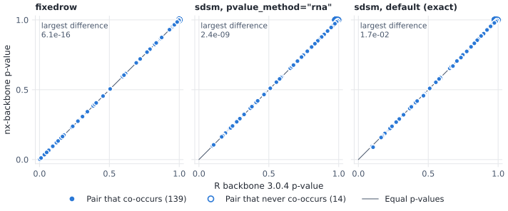
pvalue_method="rna"the p-values equal Rbackbone::sdsmup to the BiCM fit (1e-8), except that a pair that never co-occurs gets the exact value 1 (R evaluates the approximation there, but only whenmissing_as_zero = TRUE). The default uses the exact tail, which on Davis Southern Women (14 events) differs from R’s approximation by up to 0.017: the smallest p-value is 0.088 (R: 0.097), and neither finds a significant pair at alpha = 0.05. With edge constraints R estimates the probabilities of the unconstrained cells by a logistic regression on the row and column sums instead of refitting the BiCM, so its expected degrees are not exactly the observed ones; on Davis with a few constraints the p-values differ by up to 0.09.References
[1]Neal, Z. P. (2014). The backbone of bipartite projections: Inferring relationships from co-authorship, co-sponsorship, co-attendance and other co-behaviors. Social Networks, 39, 84-97.
[2]Neal, Z. P., & Neal, J. W. (2023). Stochastic Degree Sequence Model with Edge Constraints (SDSM-EC) for Backbone Extraction. Complex Networks 12, 127-136.
[3]Hong, Y. (2013). On computing the distribution function for the Poisson binomial distribution. Computational Statistics & Data Analysis, 59, 41-51.
Examples
>>> import networkx as nx
>>> from nx_backbone import sdsm
>>> B = nx.davis_southern_women_graph()
>>> women = [n for n, d in B.nodes(data=True) if d["bipartite"] == 0]
>>> scored = sdsm(B, agent_nodes=women)
>>> from nx_backbone import threshold_filter
>>> backbone = threshold_filter(scored, "sdsm_pvalue", 0.05, mode="below")
>>> all("sdsm_pvalue" in data for _, _, data in backbone.edges(data=True))
True
Computational complexity estimate is
O(I (n_a + n_f) + c^2 n_f^2 + n_a^2 + sum_z d(z)^2)time andO(e_b + c^2 n_f + B) plus the n_a^2 output edgesspace.
- nx_backbone.fdsm(B, agent_nodes=None, alpha=0.05, trials=1000, seed=None, signed=False, projection='simple', projection_weight='weight', projection_directed=False, projection_max_iter=1000, projection_tol=1e-12, burn_in=None, thin=None, *, agent_labels=None, artifact_labels=None)[source]#
Score a bipartite projection using the FDSM.
The Fixed Degree Sequence Model [1] uses Monte Carlo simulation to estimate p-values. Random bipartite graphs that exactly preserve both the row sums (agent degrees) and column sums (artifact degrees) are drawn with a curveball Markov chain (
fastball()) started at the observed graph: afterburn_intrades, one sample is taken everythintrades. The p-value is(count + 1) / (trials + 1), wherecountis the number of samples whose co-occurrence is at least (for the lower tail: at most) the observed one, so it is never exactly zero. Samples are kept as sparse matrices.- Parameters:
- Bgraph or array-like
An undirected bipartite NetworkX graph, or an agents x artifacts binary incidence matrix (NumPy array, SciPy sparse array or matrix, or pandas
DataFrame).- agent_nodesiterable or None, optional (default=None)
Nodes in the “agent” partition of a graph B. If
Nonethey are inferred as inbackbone_from_projection(). Must beNonefor a matrix B.- alphafloat, optional (default=0.05)
Retained for API compatibility. This function returns the full projected graph with p-values on all edges; apply
threshold_filter()(or usebackbone_from_projection()) to select significant edges.- trialsint, optional (default=1000)
Number of Monte Carlo samples.
- seedinteger, random_state, or None (default)
Random seed for reproducibility (int,
numpy.random.Generator,numpy.random.RandomStateorNone).- signedbool, optional (default=False)
If
True, run a two-tailed test: the stored p-value becomes two-sided and a"sign"edge attribute marks significantly strong (+1) versus significantly weak (-1) co-occurrences.- projection{“simple”, “hyper”, “newman”, “probs”, “ycn”}, optional
Projection weighting assigned to each returned edge (see
bipartite_projection()).- projection_weightstr, optional (default=”weight”)
Edge attribute name for the projection weight.
- projection_directedbool, optional (default=False)
Whether to use directed projection scores. Not supported for the undirected backbone output.
- projection_max_iterint, optional (default=1000)
Maximum iterations for
projection="ycn".- projection_tolfloat, optional (default=1e-12)
Convergence tolerance for
projection="ycn".- burn_inint or None, optional (default=None)
Curveball trades before the first sample (default
10 * n_agents).- thinint or None, optional (default=None)
Curveball trades between consecutive samples (default
5 * n_agents).- agent_labels, artifact_labelssequence or None, optional
Row and column labels of a matrix B. Only valid with a matrix B.
- Returns:
- backbonegraph
Full unipartite projection among agent nodes. Each edge has an
"fdsm_pvalue"attribute and projection weights.
- Raises:
- NetworkXError
If B is not bipartite or agent_nodes is not one side of it.
- NetworkXNotImplemented
If B is directed or a multigraph.
- ValueError
If
trials < 1, burn_in / thin is negative, or a matrix B is invalid.
See also
Notes
Comparison with R backbone. R
backbone::fdsmdraws every sample independently withfastball()from the observed matrix, using 5 trades per row of the smaller side, and reportscount / trials. On Davis Southern Women that is 70 trades per sample, too few to forget the observed matrix, and its p-values are biased upward by up to about 0.03; with 100 trades per row R’s p-values match these within Monte Carlo error. Both find the same 5 significant pairs at alpha = 0.05.References
[1]Neal, Z. P., Domagalski, R., & Sagan, B. (2021). Comparing alternatives to the fixed degree sequence model. Scientific Reports, 11, 23929.
[2]Godard, K., & Neal, Z. P. (2022). fastball: A fast algorithm to sample bipartite graphs with fixed degree sequences. Journal of Complex Networks, 10(6), cnac049.
Examples
>>> import networkx as nx
>>> from nx_backbone import fdsm
>>> B = nx.davis_southern_women_graph()
>>> women = [n for n, d in B.nodes(data=True) if d["bipartite"] == 0]
>>> scored = fdsm(B, agent_nodes=women, trials=100, seed=42)
>>> from nx_backbone import threshold_filter
>>> backbone = threshold_filter(scored, "fdsm_pvalue", 0.05, mode="below")
>>> all("fdsm_pvalue" in data for _, _, data in backbone.edges(data=True))
True
Computational complexity estimate is
O(T (S d + sum_z d(z)^2) + n_a^2)time andO(e_b + nnz(R R^T) + B) plus the n_a^2 output edgesspace.
- nx_backbone.fixedfill(B, agent_nodes=None, alpha=0.05, signed=False, projection='simple', projection_weight='weight', projection_directed=False, projection_max_iter=1000, projection_tol=1e-12, *, agent_labels=None, artifact_labels=None)[source]#
Backbone from the fixed-fill null model for bipartite projections.
Under the fixed fill model (FFM) [1] every bipartite matrix with the same number of agents, artifacts and edges (filled cells) is equally likely. The co-occurrence count of every agent pair then has the same exact distribution, obtained by conditioning on how many of the filled cells fall in the pair’s two rows; the p-value is its upper tail at the observed count (and the lower tail too when
signed=True).- Parameters:
- Bgraph or array-like
An undirected bipartite NetworkX graph, or an agents x artifacts binary incidence matrix (NumPy array, SciPy sparse array or matrix, or pandas
DataFrame).- agent_nodesiterable or None, optional (default=None)
Nodes in the “agent” partition of a graph B. If
Nonethey are inferred as inbackbone_from_projection(). Must beNonefor a matrix B.- alphafloat, optional (default=0.05)
Significance level; only pairs with p-value
< alphaare kept.- signedbool, optional (default=False)
If
True, run a two-tailed test: the p-value is two-sided and a"sign"attribute marks significantly strong (+1) or weak (-1) co-occurrence.- projection{“simple”, “hyper”, “newman”, “probs”, “ycn”}, optional
Projection weighting assigned to each returned edge (see
bipartite_projection()).- projection_weightstr, optional (default=”weight”)
Edge attribute name for the projection weight.
- projection_directedbool, optional (default=False)
Not supported for the undirected backbone (raises if
True).- projection_max_iterint, optional (default=1000)
Maximum iterations for
projection="ycn".- projection_tolfloat, optional (default=1e-12)
Convergence tolerance for
projection="ycn".- agent_labels, artifact_labelssequence or None, optional
Row and column labels of a matrix B. Only valid with a matrix B.
- Returns:
- backbonegraph
Graph on the agent nodes whose edges are the significant pairs, each with a
"fixedfill_pvalue"attribute and the projection weight.
- Raises:
- NetworkXError
If B is not bipartite or agent_nodes is not one side of it.
- NetworkXNotImplemented
If B is directed or a multigraph.
- ValueError
If projection is unknown,
projection_directed=True, or a matrix B is invalid.
See also
References
[1]Neal, Z. P., Domagalski, R., & Sagan, B. (2021). Comparing alternatives to the fixed degree sequence model. Scientific Reports, 11, 23929.
Examples
>>> import networkx as nx
>>> from nx_backbone import fixedfill
>>> B = nx.davis_southern_women_graph()
>>> women = [n for n, d in B.nodes(data=True) if d["bipartite"] == 0]
>>> H = fixedfill(B, women, alpha=0.05)
>>> all(d["fixedfill_pvalue"] < 0.05 for _, _, d in H.edges(data=True))
True
Computational complexity estimate is
O(n_f^2 + n_a^2 + sum_z d(z)^2)time andO(e_b + n_f + B)space.
- nx_backbone.fixedrow(B, agent_nodes=None, alpha=0.05, signed=False, projection='simple', projection_weight='weight', projection_directed=False, projection_max_iter=1000, projection_tol=1e-12, *, agent_labels=None, artifact_labels=None)[source]#
Backbone from the fixed-row null model for bipartite projections.
Under the fixed row model (FRM) [1] each agent keeps its degree
d_iand its artifacts are a uniformly randomd_i-subset of all artifacts, so the co-occurrence of agentsiandjis exactly hypergeometric with parameters(n_artifacts, d_i, d_j).- Parameters:
- Bgraph or array-like
An undirected bipartite NetworkX graph, or an agents x artifacts binary incidence matrix (NumPy array, SciPy sparse array or matrix, or pandas
DataFrame).- agent_nodesiterable or None, optional (default=None)
Nodes in the “agent” partition of a graph B. If
Nonethey are inferred as inbackbone_from_projection(). Must beNonefor a matrix B.- alphafloat, optional (default=0.05)
Significance level; only pairs with p-value
< alphaare kept.- signedbool, optional (default=False)
If
True, run a two-tailed test and add a"sign"attribute.- projection{“simple”, “hyper”, “newman”, “probs”, “ycn”}, optional
Projection weighting assigned to each returned edge (see
bipartite_projection()).- projection_weightstr, optional (default=”weight”)
Edge attribute name for the projection weight.
- projection_directedbool, optional (default=False)
Not supported for the undirected backbone (raises if
True).- projection_max_iterint, optional (default=1000)
Maximum iterations for
projection="ycn".- projection_tolfloat, optional (default=1e-12)
Convergence tolerance for
projection="ycn".- agent_labels, artifact_labelssequence or None, optional
Row and column labels of a matrix B. Only valid with a matrix B.
- Returns:
- backbonegraph
Graph on the agent nodes whose edges are the significant pairs, each with a
"fixedrow_pvalue"attribute and the projection weight.
- Raises:
- NetworkXError
If B is not bipartite or agent_nodes is not one side of it.
- NetworkXNotImplemented
If B is directed or a multigraph.
- ValueError
If projection is unknown,
projection_directed=True, or a matrix B is invalid.
See also
Notes
With
signed=Truea pair is signed+1when its upper tail is smaller than its lower tail and-1otherwise, as in Rbackbone, so a tie is-1. Whend_iord_jis half the number of artifacts the hypergeometric law is symmetric about its meand_i d_j / n_artifacts, and a pair observed at that mean has two equal tails. They are made exactly equal, so the pair is signed-1whatever the floating-point rounding (R signs such pairs by the rounding). Its two-sided p-value is 1.References
[1]Neal, Z. P., Domagalski, R., & Sagan, B. (2021). Comparing alternatives to the fixed degree sequence model. Scientific Reports, 11, 23929.
Examples
>>> import networkx as nx
>>> from nx_backbone import fixedrow
>>> B = nx.davis_southern_women_graph()
>>> women = [n for n, d in B.nodes(data=True) if d["bipartite"] == 0]
>>> H = fixedrow(B, women, alpha=0.05)
>>> all(d["fixedrow_pvalue"] < 0.05 for _, _, d in H.edges(data=True))
True
Computational complexity estimate is
O(n_a^2 + sum_z d(z)^2)time andO(e_b + B)space.
- nx_backbone.fixedcol(B, agent_nodes=None, alpha=0.05, signed=False, projection='simple', projection_weight='weight', projection_directed=False, projection_max_iter=1000, projection_tol=1e-12, *, agent_labels=None, artifact_labels=None)[source]#
Backbone from the fixed-column null model for bipartite projections.
Under the fixed column model (FCM) [1] each artifact
kkeeps its degreec_kand its agents are a uniformly randomc_k-subset of themagents, independently across artifacts. A given pair co-occurs on artifactkwith probabilityc_k (c_k - 1) / (m (m - 1)), so the co-occurrence count is a Poisson-binomial variable with the same distribution for every pair; it is computed exactly once and its tails give the p-values.- Parameters:
- Bgraph or array-like
An undirected bipartite NetworkX graph, or an agents x artifacts binary incidence matrix (NumPy array, SciPy sparse array or matrix, or pandas
DataFrame).- agent_nodesiterable or None, optional (default=None)
Nodes in the “agent” partition of a graph B. If
Nonethey are inferred as inbackbone_from_projection(). Must beNonefor a matrix B.- alphafloat, optional (default=0.05)
Significance level; only pairs with p-value
< alphaare kept.- signedbool, optional (default=False)
If
True, run a two-tailed test and add a"sign"attribute.- projection{“simple”, “hyper”, “newman”, “probs”, “ycn”}, optional
Projection weighting assigned to each returned edge (see
bipartite_projection()).- projection_weightstr, optional (default=”weight”)
Edge attribute name for the projection weight.
- projection_directedbool, optional (default=False)
Not supported for the undirected backbone (raises if
True).- projection_max_iterint, optional (default=1000)
Maximum iterations for
projection="ycn".- projection_tolfloat, optional (default=1e-12)
Convergence tolerance for
projection="ycn".- agent_labels, artifact_labelssequence or None, optional
Row and column labels of a matrix B. Only valid with a matrix B.
- Returns:
- backbonegraph
Graph on the agent nodes whose edges are the significant pairs, each with a
"fixedcol_pvalue"attribute and the projection weight.
- Raises:
- NetworkXError
If B is not bipartite or agent_nodes is not one side of it.
- NetworkXNotImplemented
If B is directed or a multigraph.
- ValueError
If projection is unknown,
projection_directed=True, or a matrix B is invalid.
See also
Notes
The tail is the exact Poisson-binomial one; R
backbone::fixedcoluses the refined normal approximation, which differs by up to 0.008 on Davis Southern Women.fixedfillandfixedrowequal R to rounding error.References
[1]Neal, Z. P., Domagalski, R., & Sagan, B. (2021). Comparing alternatives to the fixed degree sequence model. Scientific Reports, 11, 23929.
Examples
>>> import networkx as nx
>>> from nx_backbone import fixedcol
>>> B = nx.davis_southern_women_graph()
>>> women = [n for n, d in B.nodes(data=True) if d["bipartite"] == 0]
>>> H = fixedcol(B, women, alpha=0.05)
>>> all(d["fixedcol_pvalue"] < 0.05 for _, _, d in H.edges(data=True))
True
Computational complexity estimate is
O(n_f^2 + n_a^2 + sum_z d(z)^2)time andO(e_b + n_f + B)space.
- nx_backbone.bicm(B, agent_nodes=None, return_labels=False, *, tol=1e-08, max_iter=10000, agent_labels=None, artifact_labels=None)[source]#
Estimate Bipartite Configuration Model edge probabilities.
Fits the maximum-entropy BiCM [1]:
P[i, k] = x_i y_k / (1 + x_i y_k)where the fitness parameters solvesum_k P[i, k] = r_iandsum_i P[i, k] = c_kfor the observed agent degreesrand artifact degreesc. The fixed pointx_i = r_i / sum_k y_k / (1 + x_i y_k),y_k = c_k / sum_i x_i / (1 + x_i y_k)is iterated to convergence. Degree-0 rows/columns get probability 0 and full-degree rows/columns get probability 1 (they are fixed before solving).- Parameters:
- Bgraph or array-like
An undirected bipartite NetworkX graph, or an agents x artifacts binary incidence matrix (NumPy array, SciPy sparse array or matrix, or pandas
DataFrame).- agent_nodesiterable or None, optional (default=None)
Nodes in the “agent” partition of a graph B. If
Nonethey are inferred as inbackbone_from_projection(). Must beNonefor a matrix B.- return_labelsbool, optional (default=False)
If
True, also return(agents, artifacts)labels.- tolfloat, optional (default=1e-8)
Convergence tolerance on the maximum absolute error between expected and observed degrees.
- max_iterint, optional (default=10000)
Maximum fixed-point iterations. A
RuntimeWarningis emitted if the fit has not converged.- agent_labels, artifact_labelssequence or None, optional
Row and column labels of a matrix B. Only valid with a matrix B.
- Returns:
- Pnp.ndarray
Probability matrix of shape
(n_agents, n_artifacts)whereP[i, k]is the estimated probability of an edge between agentiand artifactk. Rows and columns are ordered bystrof their labels.- (P, agents, artifacts)tuple
Returned when
return_labels=True.
- Raises:
- NetworkXError
If B is not bipartite or agent_nodes is not one side of it.
- NetworkXNotImplemented
If B is directed or a multigraph.
- ValueError
If a matrix B is not two-dimensional and binary, or its labels do not match its shape.
- Warns:
- RuntimeWarning
If the fixed point did not converge within max_iter iterations.
See also
References
[1]Saracco, F., Di Clemente, R., Gabrielli, A., & Squartini, T. (2015). Randomizing bipartite networks: the case of the World Trade Web. Scientific Reports, 5, 10595.
Examples
>>> import networkx as nx
>>> import numpy as np
>>> from nx_backbone import bicm
>>> B = nx.davis_southern_women_graph()
>>> women = [n for n, d in B.nodes(data=True) if d["bipartite"] == 0]
>>> P, agents, artifacts = bicm(B, women, return_labels=True)
>>> degrees = np.array([B.degree(a) for a in agents])
>>> bool(np.allclose(P.sum(axis=1), degrees, atol=1e-6))
True
Computational complexity estimate is
O(I c_a c_f + n_a n_f + e_b)time andO(n_a n_f)space.
- nx_backbone.fastball(matrix, n_swaps=None, seed=None)[source]#
Randomize a binary matrix while preserving row and column sums.
This is a Curveball-style randomizer commonly used for bipartite null-model generation.
- Parameters:
- matrixarray-like
Binary matrix with shape
(n_rows, n_cols).- n_swapsint or None, optional
Number of row-pair trades. Defaults to
5 * n_rows.- seedinteger, random_state, or None
Random seed for reproducibility (int,
numpy.random.Generator,numpy.random.RandomStateorNone).
- Returns:
- randomizednp.ndarray
Randomized binary matrix with preserved row/column sums.
- Raises:
- ValueError
If matrix is not two-dimensional or n_swaps is negative.
See also
References
[1]Godard, K., & Neal, Z. P. (2022). fastball: A fast algorithm to sample bipartite graphs with fixed degree sequences. Journal of Complex Networks, 10(6), cnac049.
Examples
>>> import numpy as np
>>> from nx_backbone import fastball
>>> M = np.array([[1, 0, 1], [0, 1, 1], [1, 1, 0]])
>>> S = fastball(M, seed=1)
>>> bool((S.sum(axis=0) == M.sum(axis=0)).all() and (S.sum(axis=1) == M.sum(axis=1)).all())
True
Computational complexity estimate is
O(r c + S c)time andO(r c)space.
Gallery Examples#
Method gallery
sdsm() on Davis Southern Women, keeping sdsm_pvalue < 0.05. No pair is significant at this level; R backbone agrees (see the changelog’s reference tests).
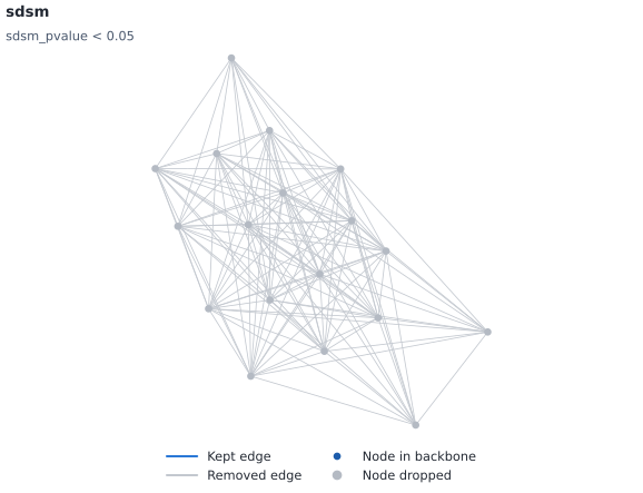
Backbone (blue) over the original graph (gray). Kept 0 of 139 edges (0%) and 0 of 18 nodes.#
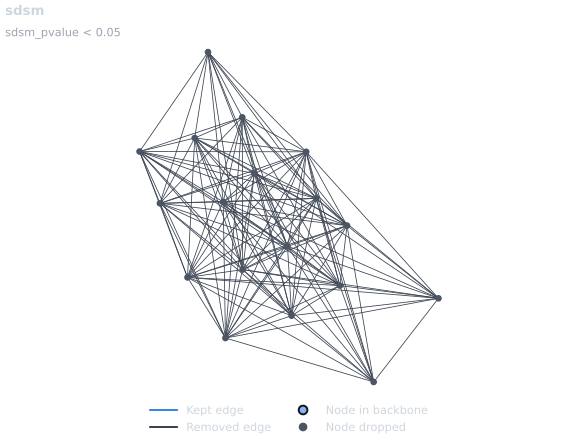
Backbone (blue) over the original graph (gray). Kept 0 of 139 edges (0%) and 0 of 18 nodes.#
fdsm() on Davis Southern Women, keeping fdsm_pvalue < 0.05.
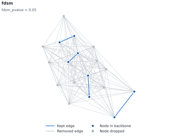
Backbone (blue) over the original graph (gray). Kept 4 of 139 edges (3%) and 8 of 18 nodes.#
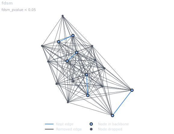
Backbone (blue) over the original graph (gray). Kept 4 of 139 edges (3%) and 8 of 18 nodes.#
fixedfill() on Davis Southern Women, keeping alpha = 0.05.
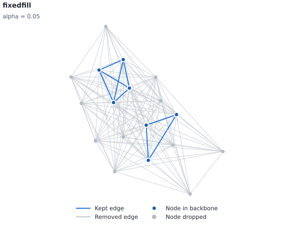
Backbone (blue) over the original graph (gray). Kept 9 of 139 edges (6%) and 7 of 18 nodes.#
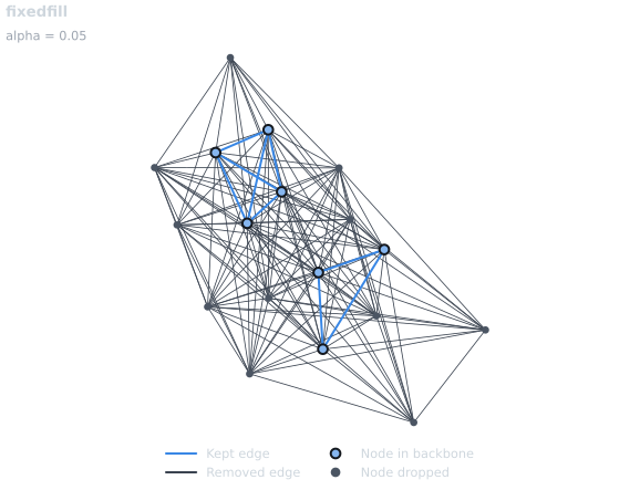
Backbone (blue) over the original graph (gray). Kept 9 of 139 edges (6%) and 7 of 18 nodes.#
fixedrow() on Davis Southern Women, keeping alpha = 0.05.
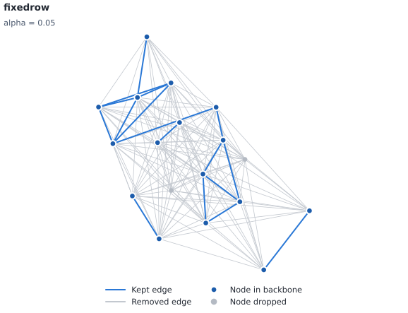
Backbone (blue) over the original graph (gray). Kept 17 of 139 edges (12%) and 16 of 18 nodes.#
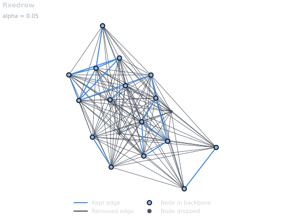
Backbone (blue) over the original graph (gray). Kept 17 of 139 edges (12%) and 16 of 18 nodes.#
fixedcol() on Davis Southern Women, keeping alpha = 0.05.
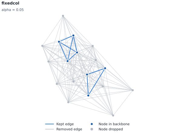
Backbone (blue) over the original graph (gray). Kept 9 of 139 edges (6%) and 7 of 18 nodes.#
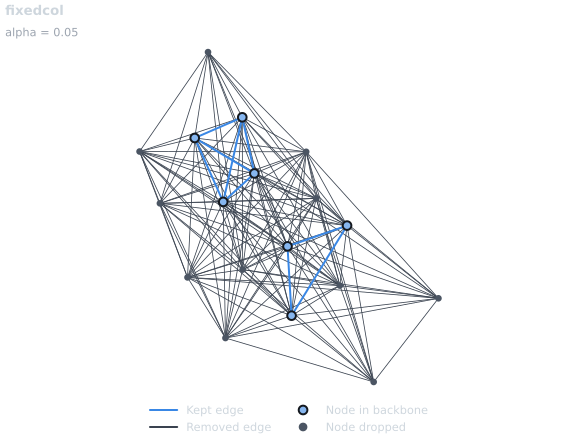
Backbone (blue) over the original graph (gray). Kept 9 of 139 edges (6%) and 7 of 18 nodes.#
fixedrow() on Davis Southern Women, keeping alpha = 0.05, signed=True.
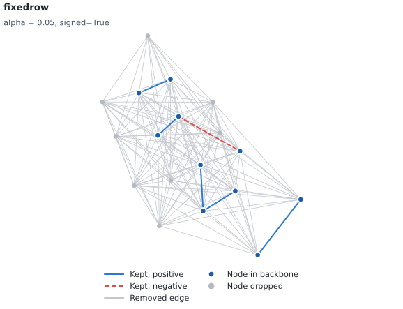
Backbone over the original graph (gray): positive edges solid blue, negative edges dashed red. Kept 6 of 139 edges (4%) and 10 of 18 nodes.#
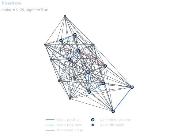
Backbone over the original graph (gray): positive edges solid blue, negative edges dashed red. Kept 6 of 139 edges (4%) and 10 of 18 nodes.#
High-Level Wrappers
- nx_backbone.backbone_from_projection(B, agent_nodes=None, method='sdsm', alpha=0.05, projection='simple', projection_weight='weight', projection_directed=False, projection_max_iter=1000, projection_tol=1e-12, mtc='none', *, missing_as_zero=True, agent_labels=None, artifact_labels=None, **kwargs)[source]#
Extract a bipartite projection backbone using method-name dispatch.
Mirrors
backbone::backbone_from_projectionin R: the selected null model scores every agent pair, the optional multiple-testing correction mtc is applied across all tested pairs (every pair unlessmissing_as_zero=False), and the pairs with (adjusted) p-value< alphaare returned. The result is thresholded the same way for every method. Pairs are scored in blocks of agent rows and only the significant ones become edges, so memory stays bounded for large projections (with mtc the p-values of all pairs are kept, 8 bytes each).- Parameters:
- Bgraph or array-like
An undirected bipartite NetworkX graph, or an agents x artifacts binary incidence matrix (NumPy array, SciPy sparse array or matrix, or pandas
DataFrame), as accepted by Rbackbone.- agent_nodesiterable or None, optional (default=None)
Nodes in the “agent” partition of a graph B. If
Nonethey are taken from thebipartitenode attribute (value 0) when present, or from a two-coloring of a connected B. Must beNonefor a matrix B, whose rows are the agents.- method{“sdsm”, “fdsm”, “fixedfill”, “fixedrow”, “fixedcol”}, optional
Null model (default
"sdsm").- alphafloat, optional (default=0.05)
Significance level for the returned backbone.
- projection{“simple”, “hyper”, “newman”, “probs”, “ycn”}, optional
Projection weighting assigned to each returned edge (see
bipartite_projection()).- projection_weightstr, optional (default=”weight”)
Edge attribute name for the projection weight.
- projection_directedbool, optional (default=False)
Not supported for the undirected backbone (raises if
True).- projection_max_iterint, optional (default=1000)
Maximum iterations for
projection="ycn".- projection_tolfloat, optional (default=1e-12)
Convergence tolerance for
projection="ycn".- mtcstring, optional (default=”none”)
Multiple-testing correction (see
adjust_pvalues()) applied to the p-values of all tested agent pairs before thresholding.- missing_as_zerobool, optional (default=True)
If
True, every agent pair is tested, including pairs that never co-occur (co-occurrence 0). IfFalse, as with Rbackbone_from_projection(whose default ismissing_as_zero = FALSE), pairs that never co-occur are not tested: they do not count toward the mtc correction and are never retained, not even as significantly weak pairs withsigned=True. The p-values of the tested pairs are the same either way. See Notes.- agent_labels, artifact_labelssequence or None, optional
Row and column labels of a matrix B (default
0, 1, ..., or aDataFrame’s index and columns). Only valid with a matrix B.- **kwargs
Passed to the selected model (e.g.
signed,trials,seed,prohibited,required,pvalue_method). SDSM-EC constraints followsdsm(): pairs that contradict B are ignored with aRuntimeWarning.
- Returns:
- backbonegraph
Graph on the agent nodes containing the significant pairs, each with a
"<method>_pvalue"attribute (unadjusted), the projection weight and, forsigned=True, a"sign"attribute.
- Raises:
- ValueError
If method is unknown or a matrix B is invalid.
- NetworkXError
If B is not bipartite or agent_nodes is not one side of it, or an SDSM-EC constraint names nodes that are not an
(agent,
artifact)
pair of B or is both required and prohibited.- AmbiguousSolution
If agent_nodes is
Noneand B is disconnected withoutbipartitenode attributes.- NetworkXNotImplemented
If B is directed or a multigraph.
Notes
By default (
missing_as_zero=True) every agent pair counts as a test for mtc, including pairs that never co-occur; Rbackbone_from_projectionwith its defaultmissing_as_zero = FALSEcounts only co-occurring pairs, so its correction is less strict when some pairs never meet. Likewise, withsigned=Truea pair that never co-occurs can be significantly weak here but is never tested by R.missing_as_zero=Falsereproduces R’s default;missing_as_zero=Truereproduces R’smissing_as_zero = TRUE. Without mtc and withsigned=Falsethe two settings give the same backbone, because a pair that never co-occurs has upper-tail p-value 1. When both tails are exactly equal the pair is signed-1, as in R.Examples
>>> import networkx as nx
>>> from nx_backbone import backbone_from_projection
>>> B = nx.davis_southern_women_graph()
>>> H = backbone_from_projection(B, method="sdsm", alpha=0.05)
>>> all(d["sdsm_pvalue"] < 0.05 for _, _, d in H.edges(data=True))
True
An incidence matrix gives the same backbone:
>>> women = sorted((n for n, d in B.nodes(data=True) if d["bipartite"] == 0), key=str)
>>> events = sorted((n for n, d in B.nodes(data=True) if d["bipartite"] == 1), key=str)
>>> M = nx.bipartite.biadjacency_matrix(B, row_order=women, column_order=events)
>>> H2 = backbone_from_projection(
...     M, method="sdsm", alpha=0.05, agent_labels=women, artifact_labels=events
... )
>>> sorted(H2.edges()) == sorted(H.edges())
True
With
missing_as_zero=Falseonly the pairs that co-occur count toward the Bonferroni correction, as in R:>>> all_pairs = backbone_from_projection(B, method="fixedfill", alpha=0.06, mtc="bonferroni") >>> cooccurring = backbone_from_projection( ... B, method="fixedfill", alpha=0.06, mtc="bonferroni", missing_as_zero=False ... ) >>> all_pairs.number_of_edges(), cooccurring.number_of_edges() (0, 1)
Computational complexity estimate is
Cost of the selected modeltime andO(e_b + B + kept edges); O(n_a^2) floats with mtcspace.
- nx_backbone.backbone_from_weighted(G, method='disparity', weight='weight', alpha=0.05, signed=False, mtc='none', collapse_multiedges=True, edge_type_attr=None, missing_as_zero=False, *, nodelist=None, directed=False, source='source', target='target', **kwargs)[source]#
Extract a weighted-network backbone using method-name dispatch.
Multi-edge inputs can be collapsed automatically before scoring.
- Parameters:
- Ggraph, array-like, sparse array or DataFrame
A weighted NetworkX graph, a weighted adjacency matrix (NumPy array or SciPy sparse array or matrix), or a pandas edge-list
DataFrame; non-graph input is converted withto_graph().- method{“disparity”, “mlf”, “lans”, “global”}, optional
Backbone method (aliases such as
"disparity_filter"accepted).- weightstring, optional (default=”weight”)
Edge weight attribute (and the edge-list column or attribute that holds the matrix entries for non-graph G).
- alphafloat, optional (default=0.05)
Significance level for the statistical methods.
- signedbool, optional (default=False)
If
True, use a two-tailed test (fordisparity/mlf/lans) so the backbone retains significantly strong and significantly weak edges, each annotated with a"sign"attribute.- mtcstring, optional (default=”none”)
Multiple-testing correction applied before thresholding (see
adjust_pvalues()).- collapse_multiedgesbool, optional (default=True)
If
TrueandGis aMultiGraphorMultiDiGraph, collapse parallel edges usingmultigraph_to_weighted().- edge_type_attrstring or None, optional (default=None)
Edge attribute used when collapsing multi-edges. If provided, edge weights count distinct edge types per node pair; otherwise they count parallel edges.
- missing_as_zerobool, optional (default=False)
If
True, every pair of distinct nodes without an edge is tested as an edge of weight 0, as withmissing_as_zero=TRUEin the R backbone package (version 3.0), and the significant ones are returned as edges with weight 0. Withsigned=Truethis keeps pairs that interact significantly less than expected (sign-1). The tested pairs also count toward themtccorrection. As in R, the"disparity"and"lans"nulls give a weight of 0 a lower-tail p-value of 0, so they keep every absent pair they can test (for"disparity", except pairs of two degree-1 nodes);"mlf"gives a graded binomial test. See the Notes ofdisparity_filter(),marginal_likelihood_filter()andlans_filter()for how each model scores them. Not supported formethod="global".- nodelistsequence or None, optional (default=None)
Node labels for the rows and columns of an adjacency matrix G.
- directedbool, optional (default=False)
Read an adjacency matrix or edge list G as a directed graph; if
Falsean adjacency matrix must be symmetric.- source, targetstr, optional (default=”source”, “target”)
Columns of an edge-list G holding the endpoints of each edge.
- **kwargs
threshold=...formethod="global".
- Returns:
- backbonegraph
The filtered graph.
- Raises:
- ValueError
If method is unknown,
method="global"lacksthreshold,missing_as_zero=Trueis combined withmethod="global", or a non-graph G is invalid (seeto_graph()).
- Warns:
- RuntimeWarning
If
missing_as_zero=Truewould test more than one million absent node pairs.
Notes
nodelist, directed, source and target only apply to non-graph input; a NetworkX graph is used as given.
Examples
>>> import networkx as nx
>>> from nx_backbone import backbone_from_weighted
>>> G = nx.les_miserables_graph()
>>> H = backbone_from_weighted(G, method="disparity", alpha=0.05)
>>> H.number_of_edges() <= G.number_of_edges()
True
A SciPy sparse adjacency matrix gives the same backbone:
>>> nodes = list(G)
>>> A = nx.to_scipy_sparse_array(G, nodelist=nodes)
>>> H2 = backbone_from_weighted(A, method="disparity", nodelist=nodes)
>>> dict(H2.edges) == dict(H.edges)
True
With
missing_as_zero=Trueandsigned=True, pairs of strong nodes that never interact are kept as significantly weak, with weight 0:>>> G = nx.Graph() >>> G.add_weighted_edges_from([("a", "b", 20), ("c", "d", 20), ("a", "c", 1)]) >>> S = backbone_from_weighted(G, method="mlf", signed=True, missing_as_zero=True) >>> sorted((u, v, d["sign"]) for u, v, d in S.edges(data=True) if d["weight"] == 0) [('a', 'd', -1), ('b', 'c', -1), ('b', 'd', -1)]
Computational complexity estimate is
O(m log n)time andO(n + m)space.
- nx_backbone.backbone_from_unweighted(G, method='sparsify', *, nodelist=None, directed=False, source='source', target='target', **kwargs)[source]#
Extract an unweighted-network backbone using method-name dispatch.
- Parameters:
- Ggraph, array-like, sparse array or DataFrame
An unweighted NetworkX graph, an adjacency matrix (NumPy array or SciPy sparse array or matrix; every nonzero entry is an edge), or a pandas edge-list
DataFrame; non-graph input is converted withto_graph(), without edge weights.- method{“sparsify”, “lspar”, “local_degree”}, optional
Sparsification method (default
"sparsify").- nodelistsequence or None, optional (default=None)
Node labels for the rows and columns of an adjacency matrix G.
- directedbool, optional (default=False)
Read an adjacency matrix or edge list G as a directed graph; if
Falsean adjacency matrix must be symmetric.- source, targetstr, optional (default=”source”, “target”)
Columns of an edge-list G holding the endpoints of each edge.
- **kwargs
Passed to the selected method (e.g.
sfor"lspar").
- Returns:
- backbonegraph
Graph containing the retained edges.
- Raises:
- ValueError
If method is unknown or a non-graph G is invalid (see
to_graph()).
See also
Notes
nodelist, directed, source and target only apply to non-graph input; a NetworkX graph is used as given.
Examples
>>> import networkx as nx
>>> from nx_backbone import backbone_from_unweighted
>>> G = nx.karate_club_graph()
>>> H = backbone_from_unweighted(G, method="lspar", s=0.5)
>>> H.number_of_nodes() == G.number_of_nodes()
True
The same backbone from a NumPy adjacency matrix:
>>> A = nx.to_numpy_array(G, weight=None)
>>> H2 = backbone_from_unweighted(A, method="lspar", s=0.5, nodelist=list(G))
>>> sorted(H2.edges()) == sorted(H.edges())
True
Computational complexity estimate is
O(mn)time andO(n + m)space.
- nx_backbone.backbone(G, method=None, **kwargs)[source]#
Unified dispatch wrapper across projection, weighted, and unweighted methods.
- Parameters:
- Ggraph, array-like, sparse array or DataFrame
A NetworkX graph; a matrix (NumPy array, SciPy sparse array or matrix, or pandas
DataFrame); or a pandas edge-listDataFrame. A matrix is read as an agents x artifacts incidence matrix for the projection methods (and when method isNone), and as an adjacency matrix for the weighted and unweighted methods. ADataFramewith the source and target columns (default"source"and"target") is an edge list. Non-graph input to the weighted and unweighted methods is converted withto_graph().- methodstring or None, optional (default=None)
Any method name accepted by
backbone_from_projection(),backbone_from_weighted()orbackbone_from_unweighted(). IfNone, the method family is chosen from G: incidence matrices and undirected simple graphs withbipartitenode attributes use the SDSM projection backbone, graphs (and edge lists) with weight edge attributes (default"weight") use the disparity filter, and other graphs usesparsify.- **kwargs
Passed to the selected wrapper (e.g.
alpha,agent_nodes,mtc,signed, the SDSM-EC constraintsprohibitedandrequired(contradictory pairs are ignored with a warning, seesdsm()), or the conversion optionsnodelist,directed,sourceandtarget).
- Returns:
- backbonegraph
The extracted backbone.
- Raises:
- ValueError
If method is not recognized, or non-graph G is invalid.
Examples
>>> import networkx as nx
>>> from nx_backbone import backbone
>>> B = nx.davis_southern_women_graph()
>>> H = backbone(B, alpha=0.05)  # bipartite attributes -> SDSM
>>> all(d["sdsm_pvalue"] < 0.05 for _, _, d in H.edges(data=True))
True
Naming a weighted method reads a matrix as a weighted adjacency matrix:
>>> G = nx.les_miserables_graph()
>>> A = nx.to_scipy_sparse_array(G, nodelist=list(G))
>>> H = backbone(A, method="disparity", nodelist=list(G))
>>> dict(H.edges) == dict(backbone(G, method="disparity").edges)
True
Computational complexity estimate is
O(n + m) dispatch checks + selected method costtime andO(1) additional beyond selected methodspace.