Visualization#
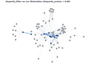
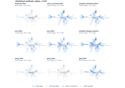
Examples in this module use nx.les_miserables_graph().
Complexity classes are provided in each function docstring.
Visualization utilities for backbone comparisons.
These helpers compare an original graph with a backbone graph and render the differences using consistent defaults:
removed nodes in red
retained edges in thicker black
- nx_backbone.graph_difference(original, backbone)[source]#
Compute node/edge overlap and removals between two graphs.
- Parameters:
- originalgraph
Reference graph.
- backbonegraph
Candidate backbone graph to compare against
original.
- Returns:
- diffdict
Dictionary containing:
"kept_nodes": nodes of original also in backbone"removed_nodes": nodes of original missing from backbone"kept_edges": edges of original also in backbone"removed_edges": edges of original missing from backbone
Edges are tuples; for undirected graphs each edge appears once with its endpoints in a canonical order.
Examples
>>> import networkx as nx
>>> from nx_backbone import graph_difference
>>> G = nx.path_graph(4)
>>> backbone = nx.Graph([(1, 0)])
>>> backbone.add_node(2)
>>> diff = graph_difference(G, backbone)
>>> diff["removed_nodes"], diff["kept_edges"]
({3}, {(0, 1)})
>>> sorted(diff["removed_edges"])
[(1, 2), (2, 3)]
Computational complexity estimate is
O(n + m)time andO(n + m)space.
- nx_backbone.compare_graphs(original, backbone, pos=None, ax=None, with_labels=False, node_size=220, kept_node_color='#f2f2f2', removed_node_color='red', base_edge_color='#c9c9c9', kept_edge_color='black', base_edge_width=0.8, kept_edge_width=2.6, title=None, return_diff=False, seed=None)[source]#
Visualize differences between an original graph and a backbone graph.
Original edges are drawn as a thin gray layer, edges retained in the backbone are drawn on top in thicker black, and nodes missing from the backbone are drawn in red.
- Parameters:
- originalgraph
Reference graph.
- backbonegraph
Backbone graph to compare against
original.- posdict or None, optional (default=None)
Node-position dictionary. If
None, usesnx.spring_layout(original, seed=seed). Pass the same pos to several calls to draw comparable panels.- axmatplotlib Axes or None, optional (default=None)
Axis to draw on. If
None, a new figure and axis are created withplt.subplots; the caller owns (and should close) it.- with_labelsbool, optional (default=False)
Whether to draw node labels.
- node_sizeint, optional (default=220)
Node size.
- kept_node_colorcolor, optional
Color for nodes retained in the backbone.
- removed_node_colorcolor, optional (default=”red”)
Color for nodes removed from the backbone.
- base_edge_colorcolor, optional
Base color for original edges.
- kept_edge_colorcolor, optional (default=”black”)
Color for retained backbone edges.
- base_edge_widthfloat, optional
Width for base/original edge layer.
- kept_edge_widthfloat, optional (default=2.6)
Width for retained backbone edges (drawn on top).
- titlestr or None, optional
Plot title.
- return_diffbool, optional (default=False)
If
True, return the computed graph-difference dictionary.- seedinteger, random_state, or None (default)
Seed for the spring layout used when pos is
None. Pass an integer for a reproducible layout.
- Returns:
- (fig, ax) or (fig, ax, diff)
Matplotlib figure/axes, and optionally the difference dictionary returned by
graph_difference().
Notes
The function never calls
plt.show().Examples
>>> import matplotlib
>>> matplotlib.use("Agg")
>>> import matplotlib.pyplot as plt
>>> import networkx as nx
>>> from nx_backbone import boolean_filter, compare_graphs, metric_backbone
>>> G = nx.les_miserables_graph()
>>> backbone = boolean_filter(metric_backbone(G), "metric_keep")
>>> fig, ax = plt.subplots()
>>> fig2, ax2 = compare_graphs(G, backbone, ax=ax, seed=1, title="Metric backbone")
>>> fig2 is fig, ax.get_title()
(True, 'Metric backbone')
>>> plt.close(fig)
Computational complexity estimate is
O(n + m) without layout; plus layout cost if pos is Nonetime andO(n + m)space.
- nx_backbone.save_graph_comparison(original, backbone, output_path, pos=None, dpi=180, bbox_inches='tight', **kwargs)[source]#
Save a comparison visualization to disk.
Draws the comparison with
compare_graphs()and writes it withFigure.savefig.- Parameters:
- originalgraph
Reference graph.
- backbonegraph
Backbone graph to compare against
original.- output_pathstr or path-like
Destination file; the format is inferred from the extension (e.g.
.png,.pdf,.svg).- posdict or None, optional (default=None)
Node positions, passed to
compare_graphs().- dpifloat, optional (default=180)
Resolution passed to
savefig.- bbox_inchesstr or None, optional (default=”tight”)
Bounding-box option passed to
savefig.- **kwargs
Further keyword arguments for
compare_graphs()(e.g.ax,title,with_labels,seed,return_diff).
- Returns:
- output_path or (output_path, diff)
The path that was written, plus the
graph_difference()dictionary whenreturn_diff=True.
Notes
If no
axis given, the figure created internally is closed after saving, so repeated calls do not accumulate open figures. A figure owned by the caller (passed viaax) is left open.Examples
>>> import os, tempfile
>>> import matplotlib
>>> matplotlib.use("Agg")
>>> import networkx as nx
>>> from nx_backbone import save_graph_comparison
>>> G = nx.cycle_graph(5)
>>> backbone = nx.path_graph(5)
>>> path = os.path.join(tempfile.mkdtemp(), "comparison.png")
>>> out, diff = save_graph_comparison(G, backbone, path, seed=1, return_diff=True)
>>> os.path.exists(out), sorted(diff["removed_edges"])
(True, [(0, 4)])
Computational complexity estimate is
O(n + m) without layout; plus rendering/write costtime andO(n + m)space.