Hybrid Methods#
Examples in this module use nx.les_miserables_graph().
Methods return scored full graphs; apply
threshold_filter() to extract final backbones.
Complexity classes are provided in each function docstring.
Hybrid backbone extraction methods.
These methods combine statistical and structural approaches.
Methods#
- glab_filter
Zhang et al. (2014) – Globally and Locally Adaptive Backbone. Tests each link’s shortest-path involvement against a local, degree-dependent null model.
- nx_backbone.glab_filter(G, weight='weight', c=0.5)[source]#
Compute GLAB (Globally and Locally Adaptive Backbone) p-values.
The GLAB method [1] (called GLANB in the paper) combines global and local information. For every node i and incident link (i, j) it computes the involvement of the link: the fraction of shortest paths from i to every other node that leave i through (i, j),
\[I_{ij} = \frac{1}{N - 1} \sum_{s \neq i} \frac{g_{is}(i, j)}{g_{is}},\]where \(g_{is}\) is the number of shortest paths between i and s and \(g_{is}(i, j)\) the number of those that use link (i, j). Link lengths are
1 / weight, so heavy links are short. Involvements sum to one over each node’s links. Under a null model in which a node’s involvement is spread uniformly over its \(k_i\) links, the statistical importance is\[SI_{ij} = (1 - I_{ij})^{(k_i - 1)^c}, \qquad k_i \geq 2,\]and the p-value of an undirected link is \(\min(SI_{ij}, SI_{ji})\). When one endpoint has degree 1, only the other endpoint’s value is used.
For a directed graph the paper (Section 2.3, Eqs. 5-6) splits each link (i, j) into an out-link of i and an in-link of j. The out-involvement \(I^{(out)}_{ij}\) is the fraction of shortest paths from i that leave through (i, j), normalized by the number of nodes reachable from i; the in-involvement \(I^{(in)}_{ij}\) is the fraction of shortest paths to j that arrive through (i, j), normalized by the number of nodes that can reach j. Then
\[SI^{(out)}_{ij} = (1 - I^{(out)}_{ij})^{(k^{(out)}_i - 1)^c}, \qquad SI^{(in)}_{ij} = (1 - I^{(in)}_{ij})^{(k^{(in)}_j - 1)^c},\]each defined when the degree in its exponent is at least 2, and the p-value of the directed link is the minimum of the two.
- Parameters:
- Gnetworkx.Graph or networkx.DiGraph
A NetworkX graph, directed or undirected.
- weightstring or None, optional (default=”weight”)
Edge attribute holding positive weights; shortest paths use
1 / weightas link length. IfNone, every link has length 1.- cfloat, optional (default=0.5)
Non-negative exponent controlling how strongly the degree of a node enters the null model.
c=0ignores degree.
- Returns:
- Hnetworkx.Graph or networkx.DiGraph
A copy of G with a
"glab_pvalue"edge attribute.
- Raises:
- NetworkXNotImplemented
If G is a multigraph.
- NetworkXError
If
weightis given and an edge has a missing, non-positive, or non-finite weight.- ValueError
If
cis negative.
See also
disparity_filterPurely local significance test.
high_salience_skeletonPurely global shortest-path-tree method.
Notes
In a disconnected graph the involvement of node i is normalized by the number of nodes reachable from i rather than \(N - 1\), so the involvements of each node still sum to one. A link whose endpoints both have degree 1 (an isolated dyad) has no null distribution and gets a p-value of 1.
In a directed graph, \(I^{(out)}\) is computed by a shortest-path search from i along out-links and \(I^{(in)}\) by a search from j along reversed links. A link whose source has out-degree below 2 uses only \(SI^{(in)}\), one whose target has in-degree below 2 uses only \(SI^{(out)}\), and a link with neither gets a p-value of 1, which mirrors the undirected degree-1 rule. On a symmetric directed graph (every link present in both directions with equal weight), out- and in-involvement of (i, j) equal the undirected \(I_{ij}\) and \(I_{ji}\), so both directions of each link get the undirected p-value.
Comparison with netbone. netbone’s
glanbcounts shortest paths: a target reached by g tied paths weighs g times in the involvement, whose denominator is the total number of paths. Here every reachable target weighs the same, as in the formula above. The two agree when no shortest paths tie.References
[1]Zhang, X., Zhang, Z., Zhao, H., Wang, Q., & Zhu, J. (2014). Extracting the globally and locally adaptive backbone of complex networks. PLoS ONE, 9(6), e100428. https://doi.org/10.1371/journal.pone.0100428
Examples
>>> import networkx as nx
>>> from nx_backbone import glab_filter, threshold_filter
>>> G = nx.les_miserables_graph()
>>> H = glab_filter(G)
>>> backbone = threshold_filter(H, "glab_pvalue", 0.05, mode="below")
>>> backbone.number_of_edges() <= H.number_of_edges()
True
Computational complexity estimate is
O(n m + n^2 log n)time andO(n k_max + m)space.
Gallery Examples#
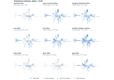
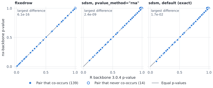
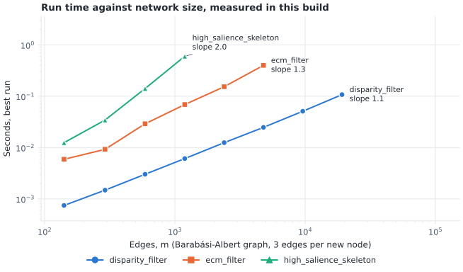
Method gallery
glab_filter() on Les Misérables, keeping glab_pvalue < 0.05.
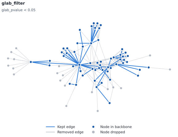
Backbone (blue) over the original graph (gray). Kept 56 of 254 edges (22%) and 57 of 77 nodes.#
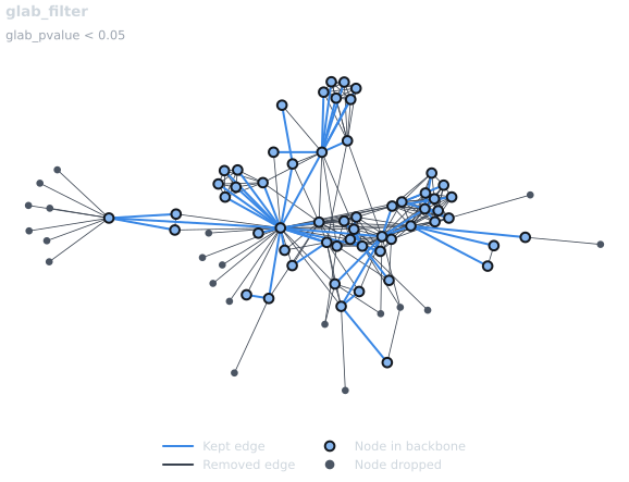
Backbone (blue) over the original graph (gray). Kept 56 of 254 edges (22%) and 57 of 77 nodes.#