Coming from R backbone or netbone

You have a backbone from the R package backbone or from the Python package netbone, perhaps in a published paper or in a colleague’s script, and you want the same result from nx-backbone. This guide maps each of their functions to ours, says where the results match exactly and where they differ by design, names the options that reproduce R, and then reproduces one R backbone on the Davis Southern Women data, p-value by p-value.

R is not installed in the documentation build. Instead, the R results come from a fixture: a file of outputs that R backbone wrote once (tests/fixtures/r_backbone.json, made by scripts/make_reference_fixtures.R). The test suite compares against the same file on every change, so what this page shows is what the tests check.

Why reproduce a reference at all

A backbone is a set of edges chosen by a test or a rule, so it is a result, not a picture. Moving a project from one tool to another should not change it. When two independent implementations (separately written programs) of the same model agree on every p-value, that is good evidence that both are right. When they disagree, you want to know whether it is a bug or a documented convention: a choice the method leaves open, such as whether a threshold keeps w > t or w >= t.

The R package is described by Neal (2022) and netbone by Yassin et al. (2023). The versions checked here are pinned in the fixtures’ metadata, which the next cell reads.

import json
import math
from pathlib import Path

import matplotlib.pyplot as plt
import networkx as nx
import numpy as np
from _figures import style
from matplotlib.lines import Line2D

import nx_backbone as nb

DOCS = Path(style.__file__).resolve().parents[1]
FIXTURES = DOCS.parent / "tests" / "fixtures"
# Figures are written as light and dark SVG pairs next to the gallery's own
# images; the page shows the one that matches the reader's theme.
OUT = DOCS / "auto_examples" / "r_and_scale" / "images"

R = json.loads((FIXTURES / "r_backbone.json").read_text(encoding="utf-8"))
NETBONE = json.loads((FIXTURES / "netbone.json").read_text(encoding="utf-8"))
meta = R["meta"]
print(
    f"R {meta['R']}, backbone {meta['backbone']}, fixture generated {meta['generated']}"
)
print(f"netbone {NETBONE['meta']['netbone']}")

R 4.3.3, backbone 3.0.4, fixture generated 2026-11-01
netbone 0.2.3

The function map: R backbone 3.0

R backbone 3.0 is organized by input type, and so are our wrappers. The model is R’s model= and our method=; R’s parameter= is our threshold= (global threshold) or s= (sparsification). The arguments alpha, signed, mtc and missing_as_zero have the same names and meanings, and mtc takes R’s p.adjust names ("bonferroni", "holm", "BH", …).

R backbone 3.0	nx-backbone	Agreement on the fixtures
backbone_from_weighted(W, model = "disparity")	backbone_from_weighted() with method="disparity", or disparity_filter()	Equal p-values and backbones; the signed lower tail differs (convention 1 below)
model = "mlf"	marginal_likelihood_filter()	Equal, signed or not
model = "lans"	lans_filter()	Equal, signed or not, including the signs of ties
model = "global", parameter = t	global_threshold_filter()	R keeps w > t, we keep w >= t (convention 4)
backbone_from_projection(I, model = "sdsm")	backbone_from_projection(), or sdsm()	Equal with pvalue_method="rna"; the default is the exact tail
model = "fixedfill", "fixedrow"	fixedfill(), fixedrow()	Equal (both exact)
model = "fixedcol"	fixedcol()	We use the exact tail, R an approximation; same backbones
model = "fdsm"	fdsm()	Equal within Monte Carlo error
SDSM-EC (structural zeros and ones)	sdsm(prohibited=..., required=...)	Different fit of the null model; same backbones
backbone_from_unweighted(U, model = "lspar", parameter = s)	lspar()	Equal with convention="r" (convention 3)
model = "degree"	local_degree()	Equal
backbone(), bicm(), fastball()	backbone(), bicm(), fastball()	bicm equal to 1e-7
stats::p.adjust()	adjust_pvalues()	Equal
the backbone object’s narrative	describe_backbone()	Methods text and citations

Our functions take a NetworkX graph or, like R, a matrix: an adjacency matrix for the weighted and unweighted wrappers (through to_graph()) and an agents-by-artifacts incidence matrix for the projection models, with agent_labels and artifact_labels for the row and column names.

The function map: netbone

netbone is a Python package with one function per method. Its p-values are in a p_value column; ours are edge attributes on a copy of the graph (disparity_pvalue, lans_pvalue, …), and a filter such as threshold_filter() turns them into a backbone.

netbone	nx-backbone	Agreement on the fixtures
disparity, lans, marginal_likelihood	disparity_filter(), lans_filter(), marginal_likelihood_filter()	Equal
metric_distance_backbone, ultrametric_distance_backbone	metric_backbone(), ultrametric_backbone()	Equal
ecm	ecm_filter()	Equal to about 1e-5, the solvers’ tolerance
noise_corrected	noise_corrected_filter()	Same score formulas with a different total weight. Both default to binomial p-values, but netbone’s count fewer trials and give \(P(X > w)\), so the backbones differ (see the Notes)
glanb	glab_filter()	Equal where no shortest paths tie
high_salience_skeleton	high_salience_skeleton()	Equal where no shortest paths tie; we split the credit of ties
h_backbone	h_backbone()	Same h-strength edges; different bridge values
mlam	multiple_linkage_analysis()	A different fitting procedure; netbone’s links are a subset of ours
doubly_stochastic	doubly_stochastic_filter()	Not comparable: netbone’s result depends on how edges are stored

Each difference, with its measured size, is in the design note Convention differences from R backbone and netbone, and in the Notes of each function’s docstring.

Four conventions, and the switches that reproduce R

Most models agree with R out of the box. Four conventions do not, and each has a way to get R’s answer:

1. Which pairs a projection tests. R leaves a pair of agents that never co-occur untested by default (missing_as_zero = FALSE), so a multiple-testing correction counts fewer tests. We test every pair. Pass missing_as_zero=False to backbone_from_projection() to test only the pairs R tests.

2. The sign of an exact tie. In a signed backbone each kept edge is marked significantly strong (+1) or significantly weak (-1). When the two tails are exactly equal, R signs the edge -1. Since version 0.3.0 we do too, so there is nothing to set; older versions signed ties +1.

3. lspar. R’s local sparsification ranks Jaccard similarities differently and keeps floor(d ** s) edges per node, with no minimum of one (Satuluri et al., 2011, describe the rule we use by default). Pass convention="r" to lspar().

4. Global threshold. R keeps w > t; global_threshold_filter() keeps w >= t, like threshold_filter(). Pass threshold=math.nextafter(t, math.inf), the next number above t.

Some differences are kept on purpose and have no switch: the lower tail of the signed disparity filter, the exact tail of fixedcol, and how the FDSM sampler mixes. They change p-values but, on the fixtures, never a backbone at alpha = 0.05.

The next cell checks all four on the fixtures, one R backbone each: how many edges R keeps, how many we keep with the defaults, and how many with the switch. “Same edges” compares the edge sets themselves, signs included, not only their sizes.

women = R["davis"]["agents"]
B = nx.davis_southern_women_graph()


def r_edges(entries, nodes):
    """R's retained ``[i, j, sign]`` rows as a set of (pair, sign)."""
    return {(frozenset((nodes[int(i)], nodes[int(j)])), int(s)) for i, j, s in entries}


def our_edges(H):
    return {(frozenset(e), H.edges[e].get("sign", 1)) for e in H.edges}


def kept(H, attr):
    return nb.boolean_filter(H, attr)


les = nx.les_miserables_graph()
les_nodes = R["les_miserables"]["nodes"]
karate = nx.Graph(nx.karate_club_graph().edges())  # binary, as R was given
karate_nodes = [int(n) for n in R["karate"]["nodes"]]
maz = R["davis"]["missing_as_zero"]["fixedfill"]["false"]

rows = [
    (
        "1. Davis, fixedfill, Bonferroni, alpha 0.06",
        r_edges(maz["0.06"]["bonferroni"], women),
        {
            "B": B,
            "agent_nodes": women,
            "method": "fixedfill",
            "alpha": 0.06,
            "mtc": "bonferroni",
        },
        {"missing_as_zero": False},
        nb.backbone_from_projection,
    ),
    (
        "2. Les Mis, signed LANS, alpha 0.05",
        r_edges(R["les_miserables"]["lans"]["backbones"]["signed_none"], les_nodes),
        {"G": les, "method": "lans", "signed": True},
        None,
        nb.backbone_from_weighted,
    ),
    (
        "3. Karate, lspar, s = 0.5",
        r_edges(R["karate"]["unweighted"]["lspar_0.5"], karate_nodes),
        {"G": karate, "s": 0.5},
        {"convention": "r"},
        lambda **kw: kept(nb.lspar(**kw), "sparsify_keep"),
    ),
    (
        "4. Les Mis, global threshold, t = 2",
        r_edges(R["les_miserables"]["global"]["backbones"]["threshold_2"], les_nodes),
        {"G": les, "threshold": 2},
        {"threshold": math.nextafter(2, math.inf)},
        lambda **kw: kept(nb.global_threshold_filter(**kw), "global_threshold_keep"),
    ),
]


def describe(edges):
    neg = sum(s < 0 for _, s in edges)
    return f"{len(edges)}" + (f" ({neg} signed -1)" if neg else "")


for label, theirs, kwargs, switch, func in rows:
    default = our_edges(func(**kwargs))
    with_switch = our_edges(func(**{**kwargs, **switch})) if switch else default
    print(label)
    print(f"   R keeps {describe(theirs)}, our default {describe(default)}")
    if switch:
        name, value = next(iter(switch.items()))
        print(f"   with {name}={value!r}: {describe(with_switch)}")
    print(f"   same edges as R: {'yes' if with_switch == theirs else 'NO'}")

1. Davis, fixedfill, Bonferroni, alpha 0.06
   R keeps 1, our default 0
   with missing_as_zero=False: 1
   same edges as R: yes
2. Les Mis, signed LANS, alpha 0.05
   R keeps 194 (126 signed -1), our default 194 (126 signed -1)
   same edges as R: yes
3. Karate, lspar, s = 0.5
   R keeps 38, our default 61
   with convention='r': 38
   same edges as R: yes
4. Les Mis, global threshold, t = 2
   R keeps 107, our default 157
   with threshold=2.0000000000000004: 107
   same edges as R: yes

Row 2 has no switch because the tie rule is now the default: our signed LANS backbone has the same edges and the same signs as R’s, including the -1 links whose two tails tie.

A worked example: Davis Southern Women in R and in Python

The Davis Southern Women data records which of 14 social events each of 18 women attended. It is bipartite: there are two kinds of node, women (the agents) and events (the artifacts), and edges only join a woman to an event. Its projection links two women by the number of events they both attended, their co-occurrence. Of the 153 pairs of women, most share at least one event, so the projection is dense, and the question a projection backbone answers is which co-occurrences are larger than chance.

“Chance” is a null model. In the fixed row model (Neal et al., 2021) each woman keeps her number of events, but which events she attends is random, so the co-occurrence of two women has a hypergeometric distribution. A pair is kept when its observed co-occurrence is improbably high under that distribution: its p-value, the probability of a co-occurrence at least that large, is below alpha.

In R, the backbone the fixture holds is

library(backbone)
bb <- backbone_from_projection(I, model = "fixedrow", alpha = 0.05)

where I is the women-by-events incidence matrix. In Python:

bb = nb.backbone_from_projection(B, agent_nodes=women, method="fixedrow", alpha=0.05)
r_bb = r_edges(R["davis"]["fixedrow"]["backbones"]["none"], women)
print(f"nx-backbone keeps {bb.number_of_edges()} pairs; R keeps {len(r_bb)}.")
print("Same pairs:", our_edges(bb) == r_bb)

nx-backbone keeps 17 pairs; R keeps 17.
Same pairs: True

The same pairs, but a backbone is only as convincing as the p-values behind it. The fixture also stores R’s p-value for every one of the 153 pairs, so we can compare them one by one. We do it for two models: the fixed row model, whose p-value both packages compute exactly, and the stochastic degree sequence model (SDSM; Neal, 2014), whose p-value R approximates with the refined normal approximation (RNA). Our sdsm() computes the exact tail by default, on inputs of any size while that is affordable, and takes pvalue_method="rna" to match R.

pairs = [(women[i], women[j]) for i, j in R["davis"]["pairs"]]
cooccur = np.array(R["davis"]["cooccurrence"])
never = cooccur == 0


def pvalues(H, attr):
    return np.array([H.edges[e][attr] for e in pairs], dtype=float)


r_fixedrow = np.array(R["davis"]["fixedrow"]["upper"], dtype=float)
r_sdsm = np.array(R["davis"]["sdsm"]["upper"], dtype=float)
# alpha > 1 keeps every pair, so each one has a p-value to compare.
ours_fixedrow = pvalues(nb.fixedrow(B, women, alpha=1.01), "fixedrow_pvalue")
ours_rna = pvalues(nb.sdsm(B, women, pvalue_method="rna"), "sdsm_pvalue")
ours_exact = pvalues(nb.sdsm(B, women), "sdsm_pvalue")

panels = [
    ("fixedrow", r_fixedrow, ours_fixedrow, slice(None)),
    ('sdsm, pvalue_method="rna"', r_sdsm, ours_rna, ~never),
    ("sdsm, default (exact)", r_sdsm, ours_exact, ~never),
]
for title, theirs, ours, which in panels:
    gap = np.max(np.abs(ours - theirs)[which])
    print(f"{title:28s} largest difference {gap:.1e}")
print(f"{never.sum()} of {len(pairs)} pairs never co-occur.")
print(
    f"For those pairs R's RNA p-values run from {r_sdsm[never].min():.3f} to "
    f"{r_sdsm[never].max():.3f}; the exact value, ours, is "
    f"{ours_rna[never].min():.0f}."
)
print(
    f"SDSM pairs with p < 0.05: R {(r_sdsm < 0.05).sum()}, "
    f"ours (RNA) {(ours_rna < 0.05).sum()}, ours (exact) {(ours_exact < 0.05).sum()}"
)


def draw_pvalues(mode):
    p = style.palette(mode)
    fig, axes = plt.subplots(
        1, 3, figsize=(7.4, 3.2), sharex=True, sharey=True, layout="constrained"
    )
    for ax, (title, theirs, ours, which) in zip(axes, panels):
        ax.plot([0, 1], [0, 1], color=p.muted, lw=0.75, zorder=1)
        ax.scatter(
            theirs[~never],
            ours[~never],
            s=24,
            c=p.kept,
            edgecolors=p.surface,
            linewidths=1.0,
            zorder=3,
        )
        ax.scatter(
            theirs[never],
            ours[never],
            s=30,
            facecolors="none",
            edgecolors=p.kept,
            linewidths=1.2,
            zorder=2,
        )
        gap = np.max(np.abs(ours - theirs)[which])
        ax.set_title(title, fontsize=9)
        ax.text(
            0.04,
            0.96,
            f"largest difference\n{gap:.1e}",
            transform=ax.transAxes,
            va="top",
            color=p.muted,
            fontsize=8,
        )
        ax.set_xlim(-0.03, 1.03)
        ax.set_ylim(-0.03, 1.03)
        ax.set_aspect("equal")
        ax.set_xticks([0, 0.5, 1])
        ax.set_yticks([0, 0.5, 1])
        ax.grid(True)
    axes[0].set_ylabel("nx-backbone p-value")
    axes[1].set_xlabel(f"R backbone {meta['backbone']} p-value")
    marker = {"marker": "o", "linestyle": "", "markersize": 6}
    handles = [
        Line2D(
            [],
            [],
            markerfacecolor=p.kept,
            markeredgecolor=p.surface,
            label=f"Pair that co-occurs ({(~never).sum()})",
            **marker,
        ),
        Line2D(
            [],
            [],
            markerfacecolor="none",
            markeredgecolor=p.kept,
            markeredgewidth=1.2,
            label=f"Pair that never co-occurs ({never.sum()})",
            **marker,
        ),
        Line2D([], [], color=p.muted, lw=0.75, label="Equal p-values"),
    ]
    fig.legend(handles=handles, loc="outside lower center", ncols=3)
    return fig


_ = style.save_variants(draw_pvalues, OUT / "coming_from_r_pvalues")

fixedrow                     largest difference 6.1e-16
sdsm, pvalue_method="rna"    largest difference 2.4e-09
sdsm, default (exact)        largest difference 1.7e-02
14 of 153 pairs never co-occur.
For those pairs R's RNA p-values run from 0.976 to 0.997; the exact value, ours, is 1.
SDSM pairs with p < 0.05: R 0, ours (RNA) 0, ours (exact) 0

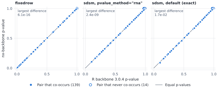
Every pair of Davis women, R’s p-value (horizontal) against ours (vertical). Points on the line are equal. The largest difference over the plotted pairs is printed in each panel; for the SDSM panels it leaves out the pairs that never co-occur (hollow circles), for which R reports an approximation and we report the exact value, 1.

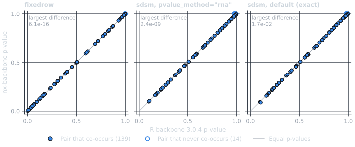
Every pair of Davis women, R’s p-value (horizontal) against ours (vertical). Points on the line are equal. The largest difference over the plotted pairs is printed in each panel; for the SDSM panels it leaves out the pairs that never co-occur (hollow circles), for which R reports an approximation and we report the exact value, 1.

Reading the three panels from left to right:

• fixedrow: both packages compute the hypergeometric tail exactly, and the p-values agree to rounding error.

• sdsm with the RNA: the same approximation, the same p-values, up to how precisely each package fits the null model’s probabilities.

• sdsm, default: our exact tail differs from R’s approximation by the printed amount. On Davis this moves no pair across alpha = 0.05 (the counts of pairs below it are printed above), so the backbones are the same; on other data they need not be. On sparse data the gap is large: when a pair’s expected co-occurrence is tiny, the RNA’s far upper tail is many orders of magnitude too small, and pure-noise pairs pass even a Benjamini-Hochberg correction (the section “Scale: sparse incidence matrices” of Bipartite projections and their backbones shows it on a planted group; issue #108). Use pvalue_method="rna" to reproduce R, and the default otherwise.

The backbone itself

Finally, here are the pairs the fixed row backbone keeps, drawn over the full projection. Every pair in it is also in R’s backbone, and the reverse.

projection = nb.simple_projection(B, women)
pos = style.layout(projection, "davis_women", weight="weight")
first_name = {w: w.split()[0] for w in women}


def draw_davis(mode):
    p = style.palette(mode)
    fig, ax = plt.subplots(figsize=(6.4, 5.6))
    counts = style.draw_backbone(
        ax,
        projection,
        bb,
        pos,
        mode=mode,
        title="Fixed row backbone of the Davis women, alpha = 0.05",
    )
    in_backbone = {n for e in bb.edges for n in e}
    for w, (x, y) in pos.items():
        ax.annotate(
            first_name[w],
            (x, y),
            xytext=(0, 7),
            textcoords="offset points",
            ha="center",
            fontsize=7.5,
            color=p.ink if w in in_backbone else p.muted,
            zorder=5,
        )
    draw_davis.caption = counts.caption
    return fig


_ = style.save_variants(draw_davis, OUT / "coming_from_r_davis")
print(draw_davis.caption)

Kept 17 of 139 edges (12%) and 16 of 18 nodes.

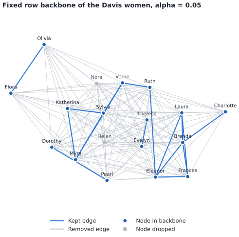
The fixed row backbone (solid blue edges) over the full co-attendance projection (faint gray edges). Women without a backbone edge are drawn in gray; the printed line above gives the counts.

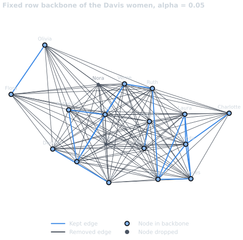
The fixed row backbone (solid blue edges) over the full co-attendance projection (faint gray edges). Women without a backbone edge are drawn in gray; the printed line above gives the counts.

A checklist for porting an R script

1. Pick the wrapper by input type, as in R: backbone_from_weighted(), backbone_from_projection() or backbone_from_unweighted(); model= becomes method=.

2. Keep alpha, signed and mtc as they are.

3. For a projection with mtc, add missing_as_zero=False to test the pairs R tests.

4. For lspar, add convention="r"; for global, use threshold=math.nextafter(t, math.inf).

5. For sdsm p-values to the digit, add pvalue_method="rna".

6. Compare edge sets, not only counts, as the table above does.

Where next

• Scaling up to large networks, the companion guide, for running these methods on large networks.

• Statistical null models side by side, for what the weighted null models assume, including signed backbones.

• The how-to tutorials Bipartite Projection Backbones and Statistical Backbone Extraction.

• Choosing a Method and Evaluating Backbones.

• The API pages Bipartite Methods, Statistical Methods and Unweighted Sparsification.

• The reference tests, tests/test_reference_implementations.py, and how to regenerate the fixtures, in Contributing.

References

• Neal, Z. P. (2014). The backbone of bipartite projections: Inferring relationships from co-authorship, co-sponsorship, co-attendance and other co-behaviors. Social Networks, 39, 84-97. https://doi.org/10.1016/j.socnet.2014.06.001

• Neal, Z. P. (2022). backbone: An R package to extract network backbones. PLoS ONE, 17(5), e0269137. https://doi.org/10.1371/journal.pone.0269137

• Neal, Z. P., Domagalski, R., & Sagan, B. (2021). Comparing alternatives to the fixed degree sequence model for extracting the backbone of bipartite projections. Scientific Reports, 11, 23929. https://doi.org/10.1038/s41598-021-03238-3

• Satuluri, V., Parthasarathy, S., & Ruan, Y. (2011). Local graph sparsification for scalable clustering. Proceedings of the ACM SIGMOD International Conference on Management of Data, 721-732. https://doi.org/10.1145/1989323.1989399

• Yassin, A., Haidar, A., Cherifi, H., Seba, H., & Togni, O. (2023). An evaluation tool for backbone extraction techniques in weighted complex networks. Scientific Reports, 13, 17000. https://doi.org/10.1038/s41598-023-42076-3