Quick Start#
This guide walks through the basic workflow of extracting a backbone from
a network using nx-backbone.
Tip
Next, read From a hairball to a backbone, end to end. This page shows the calls; that worked case study, with figures, explains why each step is needed and how to choose alpha and a multiple-testing correction, compare methods, validate the result, and report it.
Import#
The recommended import convention is:
import networkx as nx
import nx_backbone as nb
Step 1: Create or load a weighted graph#
Most backbone methods operate on weighted graphs. Here we use the built-in Les Miserables co-appearance network:
G = nx.les_miserables_graph()
Step 2: Apply a backbone method#
Apply the disparity filter to compute a p-value for each edge. This returns
a copy of the graph with an added "disparity_pvalue" edge attribute:
scored = nb.disparity_filter(G)
Step 3: Filter to extract the backbone#
Use threshold_filter() to keep only edges whose
p-value is below a significance threshold:
backbone = nb.threshold_filter(scored, "disparity_pvalue", 0.05)
Every edge gets its own test, so with hundreds of edges some will pass by
chance. Pass mtc to correct for multiple testing ("bonferroni",
"holm", "hochberg", "bh"/"fdr", or "by"):
strict = nb.threshold_filter(scored, "disparity_pvalue", 0.05, mtc="holm")
Step 4: Evaluate the backbone#
Use the measures module to compare the backbone
to the original graph:
print(f"Edges kept: {nb.edge_fraction(G, backbone):.1%}")
print(f"Nodes kept: {nb.node_fraction(G, backbone):.1%}")
Disparity filter visualization#
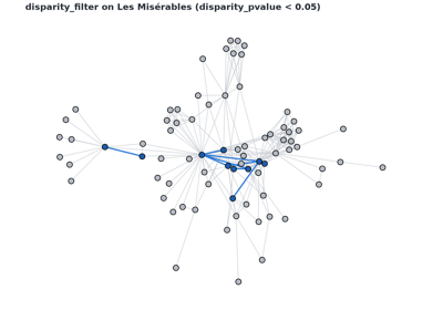
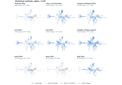
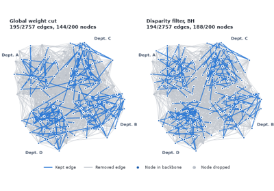
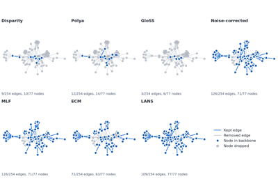
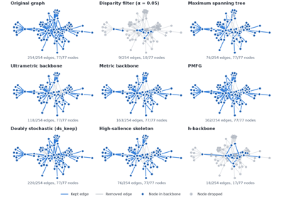
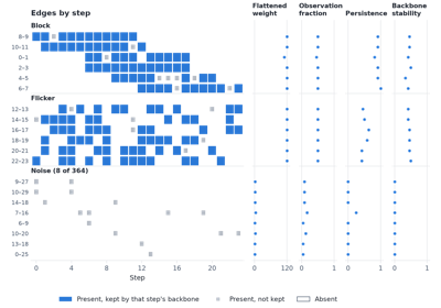
The Sphinx Gallery example below visualizes retained and removed structure
after applying disparity_filter followed by threshold_filter.
Other approaches#
Proximity-based scoring: Score edges by how structurally embedded they are using neighborhood similarity, then keep the top fraction:
scored = nb.jaccard_backbone(G)
backbone = nb.fraction_filter(scored, "jaccard", 0.2, ascending=False)
Structural backbone: Score edges by metric-backbone membership and then filter using the boolean keep attribute:
scored = nb.metric_backbone(G)
backbone = nb.boolean_filter(scored, "metric_keep")
Bipartite backbone: Score a bipartite projection, then filter by p-value:
B = nx.davis_southern_women_graph()
women_nodes = [n for n, d in B.nodes(data=True) if d["bipartite"] == 0]
scored = nb.sdsm(B, agent_nodes=women_nodes, projection="hyper")
backbone = nb.threshold_filter(scored, "sdsm_pvalue", 0.05, mode="below")
The narrative tutorial Bipartite projections and their backbones explains these choices with figures.
Hypergraph backbone: Prune nested and redundant hyperedges with the parameter-free minimum-description-length backbone:
H = [(1, 2, 3, 4), (1, 2, 3), (2, 3, 4), (8, 9)]
result = nb.mdl_hypergraph_backbone(H)
result.backbone   # [frozenset({1, 2, 3, 4}), frozenset({8, 9})]
Comparing methods: Systematically compare multiple backbones:
backbones = {
    "disparity": nb.threshold_filter(nb.disparity_filter(G), "disparity_pvalue", 0.05),
    "mst": nb.boolean_filter(nb.maximum_spanning_tree_backbone(G), "mst_keep"),
}
results = nb.compare_backbones(G, backbones)
Next steps#
From a hairball to a backbone, end to end – Start here: the whole workflow as a worked case study, with figures
Concepts – Learn about the different categories of backbone methods
User Guide – Detailed guides on workflows, method selection, and evaluation
Tutorials – Step-by-step tutorials for each method category
Coming from R backbone or netbone – Coming from R
backboneornetboneAPI Reference – Complete API reference