Scaling up to large networks

Every method in nx-backbone runs in a blink on Les Misérables (77 nodes). A network with a hundred thousand nodes is different: some methods still take seconds, others would take days or run out of memory. This guide explains which is which and what to do about it, in four steps: start from sparse data, choose a method whose cost grows slowly, know what the ECM solver does on large graphs, and use a NetworkX backend where it helps. It ends with tips for keeping memory in check.

The timings below are measured while the documentation is built, on small graphs, so that the build stays fast. They show how cost grows, not what your machine will take on your data.

Two words first. A network has n nodes and m edges. A method’s complexity, such as O(n + m), says how its running time (or memory) grows with n and m: double the edges of an O(m) method and it takes about twice as long; double them for an O(n m) method and it takes about four times as long, because n grows too.

import contextlib
import os
import platform
import re
import time
import tracemalloc
from datetime import date
from pathlib import Path

import matplotlib.pyplot as plt
import networkx as nx
import numpy as np
import scipy.sparse as sp
from _figures import style

import nx_backbone as nb

DOCS = Path(style.__file__).resolve().parents[1]
# Light and dark SVG pairs, next to the gallery's own images.
OUT = DOCS / "auto_examples" / "r_and_scale" / "images"


def weighted_graph(n, m=3, max_weight=20, seed=0):
    """The seeded Barabási-Albert graph of ``benchmarks/benchmarks/_data.py``."""
    G = nx.barabasi_albert_graph(n, m, seed=seed)
    rng = np.random.default_rng(seed)
    weights = rng.integers(1, max_weight + 1, size=G.number_of_edges())
    for (u, v), w in zip(G.edges(), weights):
        G[u][v]["weight"] = int(w)
    return G

Start from sparse data

Large networks are sparse: each node has a few neighbors, not thousands, so m is a small multiple of n. A sparse matrix stores only the nonzero entries, so its memory grows with m. A dense matrix stores all n x n entries, zeros included, and its memory grows with n squared.

If your data is already a SciPy sparse adjacency matrix, pass it straight to the wrappers: backbone_from_weighted() and backbone_from_unweighted() convert it with to_graph(), which reads only the stored entries.

G = weighted_graph(5000)
A = nx.to_scipy_sparse_array(G, weight="weight", format="csr")
from_matrix = nb.backbone_from_weighted(A, method="disparity", nodelist=list(G))
from_graph = nb.backbone_from_weighted(G, method="disparity")
print(f"{G.number_of_nodes()} nodes, {G.number_of_edges()} edges")
print(
    f"Disparity backbone from the sparse matrix: {from_matrix.number_of_edges()} "
    f"edges; from the graph: {from_graph.number_of_edges()} edges; "
    f"same edges: {set(map(frozenset, from_matrix.edges)) == set(map(frozenset, from_graph.edges))}"
)

5000 nodes, 14991 edges
Disparity backbone from the sparse matrix: 90 edges; from the graph: 90 edges; same edges: True

How much memory does each form take? tracemalloc, from the Python standard library, counts the bytes Python allocates while the graph is built. A NetworkX graph keeps a dictionary per node and per edge, which is flexible but costs far more per edge than the three arrays of a sparse matrix.

tracemalloc.start()
H = nx.from_scipy_sparse_array(A, edge_attribute="weight")
graph_bytes, _ = tracemalloc.get_traced_memory()
tracemalloc.stop()
del H
csr_bytes = A.data.nbytes + A.indices.nbytes + A.indptr.nbytes
n, m = G.number_of_nodes(), G.number_of_edges()
print(f"NetworkX graph: {graph_bytes / m:,.0f} bytes per edge")
print(f"Sparse matrix:  {csr_bytes / m:,.0f} bytes per edge (each edge stored twice)")
print(
    f"Dense matrix:   {n * n * 8 / m:,.0f} bytes per edge ({n * n * 8 / 1e6:,.0f} MB)"
)

NetworkX graph: 389 bytes per edge
Sparse matrix:  35 bytes per edge (each edge stored twice)
Dense matrix:   13,341 bytes per edge (200 MB)

The graph is still the convenient form to work in, and it is what every method returns. The point is to never go through a dense matrix on the way.

The same holds for bipartite data. The projection models, backbone_from_projection() and the functions it calls, accept an agents-by-artifacts incidence matrix (a 1 where an agent takes part in an artifact) as a NumPy array, a SciPy sparse array or a pandas DataFrame. Internally they keep it sparse and count co-occurrences one block of agent rows at a time, so no dense agents-by-agents matrix is formed.

rng = np.random.default_rng(0)
n_agents, n_artifacts = 1000, 300
incidence = sp.random_array(
    (n_agents, n_artifacts), density=0.05, format="csr", rng=rng, dtype=np.int8
)
incidence.data[:] = 1
labels = [f"agent {i}" for i in range(n_agents)]
start = time.perf_counter()
bipartite_bb = nb.backbone_from_projection(
    incidence, method="fixedfill", agent_labels=labels
)
seconds = time.perf_counter() - start
print(
    f"{n_agents} x {n_artifacts} sparse incidence ({incidence.nnz} ones): "
    f"{bipartite_bb.number_of_edges()} significant pairs of "
    f"{n_agents * (n_agents - 1) // 2} in {seconds:.2f} s"
)

1000 x 300 sparse incidence (15000 ones): 20039 significant pairs of 499500 in 0.11 s

Choose a method whose cost grows slowly

The methods fall into a few cost classes. The full list, with memory, is in Complexity Summary; the summary:

Time	Methods	At scale
O(n + m) or O(m log n)	disparity_filter(), noise_corrected_filter(), marginal_likelihood_filter(), lans_filter(), global_threshold_filter(), maximum_spanning_tree_backbone()	Time grows about in proportion to m
O(I C^2) over C classes	ecm_filter()	See the ECM section below
O(n m + n^2 log n): one shortest-path search per node	high_salience_skeleton(), metric_backbone(), edge_betweenness_filter(), h_backbone(), glab_filter()	Time grows about with m squared on sparse graphs; a backend can help some of them
O(n_a^2 n_f)	The projection models, sdsm(), fixedfill(), …; fdsm() multiplies it by its trials	Grows with the square of the number of agents
O(n^3) time, O(n^2) memory	local_path_index()	Small graphs only

Complexity classes hide constants, so here is the real thing: three methods, one from each of the first three rows, timed on the seeded Barabási-Albert graph of the benchmark suite (benchmarks/) at doubling sizes. To keep the build short, each method stops growing once a single run takes more than a third of a second. Each time is the best of up to three runs. Multithreaded linear algebra is limited to one thread when threadpoolctl is installed, because on a busy machine competing threads make the ECM fit much slower and its timing erratic.

try:
    from threadpoolctl import threadpool_limits
except ImportError:  # optional
    threadpool_limits = None

METHODS = ["disparity_filter", "ecm_filter", "high_salience_skeleton"]
SIZES = [50 * 2**k for k in range(8)]  # 50 ... 6400 nodes
STOP = 1 / 3  # seconds


def best_time(func, graph, budget=0.25):
    runs = []
    begin = time.perf_counter()
    while len(runs) < 3 and (not runs or time.perf_counter() - begin < budget):
        t0 = time.perf_counter()
        func(graph)
        runs.append(time.perf_counter() - t0)
    return min(runs)


graphs = {}
timings = {name: [] for name in METHODS}
limits = threadpool_limits(limits=1) if threadpool_limits else contextlib.nullcontext()
with limits:
    nb.ecm_filter(nx.les_miserables_graph())  # import SciPy outside the timings
    for name in METHODS:
        func = getattr(nb, name)
        for size in SIZES:
            graph = graphs.setdefault(size, weighted_graph(size))
            seconds = best_time(func, graph)
            timings[name].append((graph.number_of_edges(), seconds))
            if seconds > STOP:
                break


def slope(points):
    """Least-squares slope of log(time) against log(edges), largest 3 sizes."""
    x, y = np.log([e for e, _ in points[-3:]]), np.log([t for _, t in points[-3:]])
    return np.polyfit(x, y, 1)[0]


print(
    f"Measured {date.today():%Y-%m-%d} on {platform.machine()}, {os.cpu_count()} CPUs"
)
print(f"Python {platform.python_version()}, NetworkX {nx.__version__}")
print(f"BLAS limited to one thread: {'yes' if threadpool_limits else 'no'}")
for name, points in timings.items():
    print(f"\n{name}, slope {slope(points):.1f}")
    for e, t in points:
        print(f"  {e:7,} edges  {t * 1000:8.1f} ms")

Measured 2026-11-02 on x86_64, 4 CPUs
Python 3.12.15, NetworkX 3.7
BLAS limited to one thread: no

disparity_filter, slope 1.1
      141 edges       0.7 ms
      291 edges       1.5 ms
      591 edges       3.0 ms
    1,191 edges       6.1 ms
    2,391 edges      12.5 ms
    4,791 edges      24.8 ms
    9,591 edges      51.0 ms
   19,191 edges     107.5 ms

ecm_filter, slope 1.3
      141 edges       5.9 ms
      291 edges       9.3 ms
      591 edges      29.1 ms
    1,191 edges      68.9 ms
    2,391 edges     153.3 ms
    4,791 edges     399.8 ms

high_salience_skeleton, slope 2.0
      141 edges      12.5 ms
      291 edges      34.4 ms
      591 edges     141.3 ms
    1,191 edges     600.1 ms

The slope is the exponent of a power law fitted to each method’s three largest sizes: about 1 means the time grows in proportion to m, about 2 means it grows with m squared. The smallest sizes are left out because there fixed costs, such as copying the graph, dominate, which flattens the left end of the fastest line. Timings on a shared machine are noisy, so read the slopes as rough.

def draw_timings(mode):
    p = style.palette(mode)
    colors = style.categorical(len(METHODS), mode)
    markers = ["o", "s", "^"]
    fig, ax = plt.subplots(figsize=(6.8, 4.0), layout="constrained")
    ends = []
    for (name, points), color, marker in zip(timings.items(), colors, markers):
        edges, secs = zip(*points)
        ax.plot(
            edges,
            secs,
            color=color,
            marker=marker,
            markersize=6,
            markeredgecolor=p.surface,
            markeredgewidth=1.0,
        )
        ends.append((secs[-1], edges[-1], name, points))
    ax.set_xscale("log")
    ax.set_yscale("log")
    all_points = [pt for points in timings.values() for pt in points]
    ax.set_xlim(min(e for e, _ in all_points) / 1.5, max(e for e, _ in all_points) * 8)
    ax.set_ylim(min(t for _, t in all_points) / 2, max(t for _, t in all_points) * 6)
    # Direct labels right of each line's last point, nudged up (in points) so
    # that two lines ending at about the same time stay legible.
    to_points = 72.0 / fig.dpi
    placed = []
    for sec, edge, name, points in sorted(ends):
        y = ax.transData.transform((edge, sec))[1] * to_points
        lift = 0.0
        if placed and y - placed[-1] < 24.0:
            lift = placed[-1] + 24.0 - y
        placed.append(y + lift)
        ax.annotate(
            f"{name}\nslope {slope(points):.1f}",
            xy=(edge, sec),
            xytext=(8, lift),
            textcoords="offset points",
            va="center",
            fontsize=8,
            color=p.ink,
            # A hairline leader when the label had to move off its point.
            arrowprops={"arrowstyle": "-", "color": p.muted, "lw": 0.6, "shrinkA": 2}
            if lift
            else None,
        )
    ax.set_xlabel("Edges, m (Barabási-Albert graph, 3 edges per new node)")
    ax.set_ylabel("Seconds, best run")
    ax.set_title("Run time against network size, measured in this build")
    ax.grid(True, which="major")
    handles = [
        plt.Line2D([], [], color=c, marker=mk, markersize=6, label=name)
        for name, c, mk in zip(METHODS, colors, markers)
    ]
    fig.legend(handles=handles, loc="outside lower center", ncols=3)
    return fig


_ = style.save_variants(draw_timings, OUT / "scaling_up_timings")

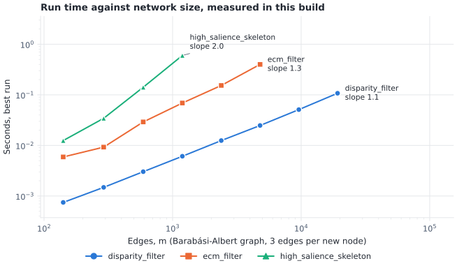
Run time against the number of edges on log-log axes, measured during this documentation build (the printed output above gives the machine and every value). Each line stops once a run takes more than a third of a second. A steeper line means a cost that grows faster.

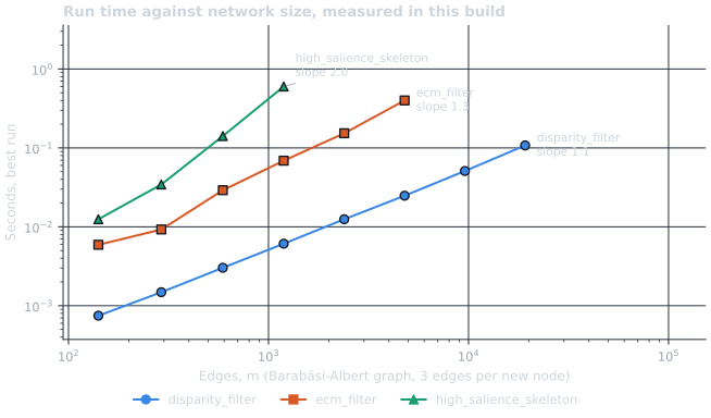
Run time against the number of edges on log-log axes, measured during this documentation build (the printed output above gives the machine and every value). Each line stops once a run takes more than a third of a second. A steeper line means a cost that grows faster.

The shortest-path methods are the ones to plan for. A slope near 2 means that ten times more edges take about a hundred times longer, so a method that takes a second at a few thousand edges takes minutes at tens of thousands and hours beyond that. The local statistical filters grow about in proportion to the edges.

The ECM solver on large graphs

The enhanced configuration model (ECM; Gemmetto et al., 2017) is the statistical null that keeps both each node’s degree and its strength (the sum of its edge weights). Fitting it means solving for two numbers per node, which used to make it the slowest statistical method by far.

Two nodes with the same degree and the same strength get the same numbers in the fitted model, so ecm_filter() solves for one pair of numbers per class of such nodes instead of per node. This is exact, not an approximation, and its cost depends on the number of classes C rather than on n. How many classes do real-sized graphs have?

class_counts = []
for size in [250, 500, 1000, 2000, 5000, 10000, 20000]:
    graph = graphs.get(size) or weighted_graph(size)
    strength = dict(graph.degree(weight="weight"))
    classes = len({(graph.degree(v), strength[v]) for v in graph})
    class_counts.append((size, classes))
    print(f"{size:6,} nodes: {classes:5,} degree-strength classes")


def draw_classes(mode):
    p = style.palette(mode)
    fig, ax = plt.subplots(figsize=(6.0, 3.8), layout="constrained")
    sizes, classes = zip(*class_counts)
    ax.plot(
        [sizes[0], sizes[-1]],
        [sizes[0], sizes[-1]],
        color=p.muted,
        lw=0.75,
    )
    ax.annotate(
        "one class per node",
        (sizes[-1], sizes[-1]),
        xytext=(-4, 4),
        textcoords="offset points",
        ha="right",
        va="bottom",
        fontsize=8,
        color=p.muted,
    )
    ax.plot(
        sizes,
        classes,
        color=p.kept,
        marker="o",
        markersize=6,
        markeredgecolor=p.surface,
        markeredgewidth=1.0,
    )
    for size, count in class_counts[-1:] + class_counts[3:4]:
        ax.annotate(
            f"{count:,} classes",
            (size, count),
            xytext=(0, -12),
            textcoords="offset points",
            ha="center",
            va="top",
            fontsize=8,
            color=p.ink,
        )
    ax.set_xscale("log")
    ax.set_yscale("log")
    ax.set_xlabel("Nodes, n")
    ax.set_ylabel("Degree-strength classes, C")
    ax.set_title("ECM fits classes, not nodes")
    ax.grid(True)
    return fig


_ = style.save_variants(draw_classes, OUT / "scaling_up_ecm_classes")

   250 nodes:   148 degree-strength classes
   500 nodes:   249 degree-strength classes
 1,000 nodes:   374 degree-strength classes
 2,000 nodes:   520 degree-strength classes
 5,000 nodes:   870 degree-strength classes
10,000 nodes: 1,204 degree-strength classes
20,000 nodes: 1,695 degree-strength classes

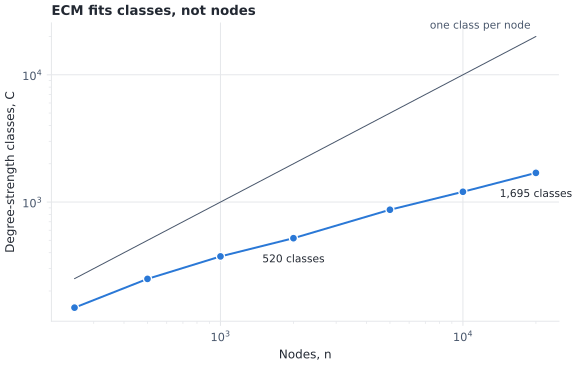
Distinct (degree, strength) classes in the seeded Barabási-Albert graphs, against the number of nodes. The gray line is one class per node, the cost before classes were used. The printed output above gives every value.

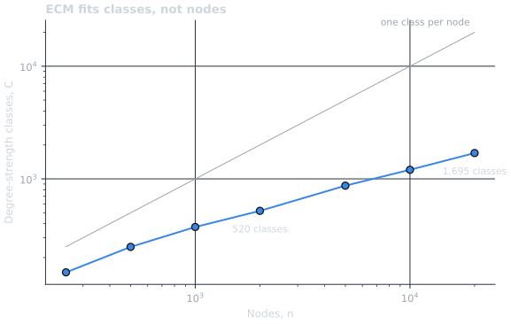
Distinct (degree, strength) classes in the seeded Barabási-Albert graphs, against the number of nodes. The gray line is one class per node, the cost before classes were used. The printed output above gives every value.

Each solver step costs about C squared operations, done in fixed-size chunks so that memory does not grow with C. Up to 4,000 parameters a step is a dense linear solve; above that, the solver switches to conjugate gradients. When this solver was introduced (pull request #53, measured on 2026-11-01 on a shared 4-core machine with one BLAS thread), a 20,000-node graph took about 16 seconds; before it, a 2,000-node graph took about 90 seconds. A directed graph has more classes, because a class is then fixed by four numbers (out- and in-degree and strength), and fits more slowly.

Weights matter too: the ECM treats weights as counts, so a graph whose weights take many distinct values has more classes. The unit= argument of ecm_filter() says how much weight one count is.

NetworkX backends

NetworkX can hand an algorithm to a backend, a separately installed package such as nx-parallel (several CPU cores) or nx-cugraph (an NVIDIA GPU). No backend implements a backbone method itself, but the shortest-path methods spend their time in NetworkX algorithms that backends do implement, such as edge betweenness. Listing a backend in nx.config.backend_priority lets those inner calls run on it:

# pip install nx-parallel
with nx.config.backend_priority(algos=["parallel"]):
    H = nb.edge_betweenness_filter(G)

These timings were not measured in this build: they are the committed measurements in Backends, read from that page here. They were recorded on 2026-11-01 with scripts/benchmark_backends.py on a 4-CPU machine (Python 3.13, NetworkX 3.7, nx-parallel 0.4), on a 1,000-node Barabási-Albert graph, best of 3 runs.

table = (DOCS / "user_guide" / "backends.rst").read_text(encoding="utf-8")
backend_rows = [
    (name, float(nx_s), float(par_s))
    for name, nx_s, par_s in re.findall(
        r"^``(\w+)``\s+([\d.]+)\s+([\d.]+)\s+[\d.]+\s+\S+\s*$", table, flags=re.M
    )
]
for name, nx_s, par_s in backend_rows:
    print(f"{name:26s} NetworkX {nx_s:5.2f} s   nx-parallel {par_s:5.2f} s")


def draw_backends(mode):
    p = style.palette(mode)
    base, parallel = style.categorical(2, mode)
    fig, ax = plt.subplots(figsize=(6.4, 3.2), layout="constrained")
    rows = sorted(backend_rows, key=lambda r: r[1] / r[2])
    for y, (_name, nx_s, par_s) in enumerate(rows):
        ax.plot([nx_s, par_s], [y, y], color=p.hairline, lw=2.0, zorder=1)
        ax.scatter(nx_s, y, s=46, marker="o", c=base, edgecolors=p.surface, zorder=3)
        ax.scatter(
            par_s, y, s=50, marker="s", c=parallel, edgecolors=p.surface, zorder=3
        )
        ax.annotate(
            f"{nx_s / par_s:.1f}x",
            (max(nx_s, par_s), y),
            xytext=(8, 0),
            textcoords="offset points",
            va="center",
            fontsize=8,
            color=p.ink,
        )
    ax.set_yticks(range(len(rows)), [r[0] for r in rows])
    ax.tick_params(axis="y", labelcolor=p.ink)
    ax.set_xlim(0, max(max(r[1], r[2]) for r in rows) * 1.18)
    ax.set_ylim(-0.6, len(rows) - 0.4)
    ax.set_xlabel("Seconds (committed measurement, not run in this build)")
    ax.set_title("NetworkX alone and with nx-parallel, 1,000 nodes")
    ax.grid(True, axis="x")
    ax.spines["left"].set_visible(False)
    handles = [
        plt.Line2D(
            [], [], marker="o", linestyle="", color=base, label="NetworkX alone"
        ),
        plt.Line2D(
            [],
            [],
            marker="s",
            linestyle="",
            color=parallel,
            label="With nx-parallel",
        ),
    ]
    fig.legend(handles=handles, loc="outside lower center", ncols=2)
    return fig


_ = style.save_variants(draw_backends, OUT / "scaling_up_backends")

metric_backbone            NetworkX  2.23 s   nx-parallel  2.13 s
edge_betweenness_filter    NetworkX  4.29 s   nx-parallel  1.13 s
h_backbone                 NetworkX  1.82 s   nx-parallel  0.54 s
high_salience_skeleton     NetworkX  3.16 s   nx-parallel  3.40 s
glab_filter                NetworkX  3.50 s   nx-parallel  3.84 s

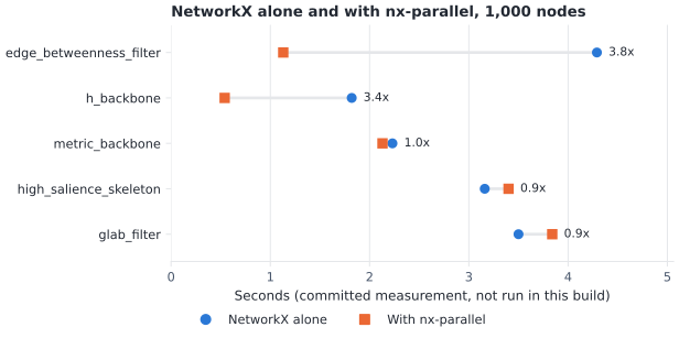
The committed nx-parallel measurements from Backends (circles: NetworkX alone; squares: with nx-parallel). The label on each row is the NetworkX time divided by the nx-parallel time.

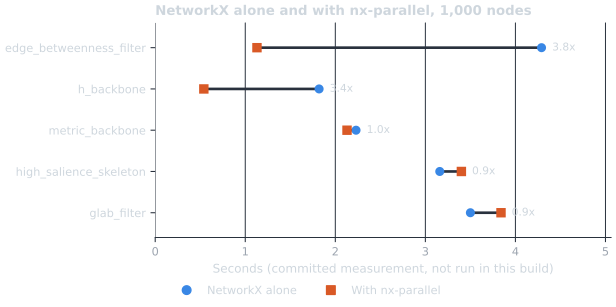
The committed nx-parallel measurements from Backends (circles: NetworkX alone; squares: with nx-parallel). The label on each row is the NetworkX time divided by the nx-parallel time.

Only the methods built on edge betweenness gain: nx-parallel implements edge betweenness, but not the single-source search that the high salience skeleton and GLAB run once per node. The results were the same with and without the backend, up to the last bits of the betweenness sums. Measure on your own graphs and hardware before relying on a speed-up.

Memory tips

• Score once, filter many times. Scoring is the expensive step; threshold_filter() on a scored graph is cheap. Keep the scored graph and try several alphas on it.

• Avoid all-pairs memory on big graphs. metric_backbone(), doubly_stochastic_filter() and local_path_index() use memory that grows with n squared (see Complexity Summary).

• Know what a scorer returns. sdsm() and fdsm() return every pair of agents with its p-value, n_a (n_a - 1) / 2 edges (for the sparse incidence above, the number of pairs printed after “of”). backbone_from_projection() returns only the significant ones.

• Testing absent pairs is quadratic. missing_as_zero=True tests every pair of nodes that is not linked as a weight-0 edge, and ecm_filter() warns when that would add more than a million edges.

• Limit threads when you run many jobs. Running several analyses side by side, each with multithreaded linear algebra, oversubscribes the CPUs. Set OPENBLAS_NUM_THREADS=1 (or use threadpoolctl) and parallelize over jobs instead.

Where next

• Complexity Summary for the complexity of every function, and Backends for backends and how to test with them.

• Coming from R backbone or netbone, the companion guide, for reproducing R backbone and netbone.

• The how-to tutorials Statistical Backbone Extraction and Bipartite Projection Backbones.

• The API pages Convert (to_graph()), Statistical Methods and Bipartite Methods.

• The asv benchmark suite in benchmarks/, described in Contributing, for timing a change.

References

• Gemmetto, V., Cardillo, A., & Garlaschelli, D. (2017). Irreducible network backbones: unbiased graph filtering via maximum entropy. arXiv:1706.00230.