Structural Methods#
Examples in this module use nx.les_miserables_graph().
These functions return scored full graphs. Extract final backbones with
boolean_filter() on *_keep flags (or
threshold_filter() for continuous scores such as
salience and ds_weight).
Complexity classes are provided in each function docstring.
Structural backbone extraction methods.
These methods use the network’s topology (edge weights, shortest paths, spanning trees, degree, neighborhood overlap) to identify the most important substructure.
Methods#
- global_threshold_filter
Simple weight cutoff.
- strongest_n_ties
Per-node strongest edges.
- global_sparsification
Keep top-weight edges globally by fraction.
- primary_linkage_analysis
Nystuen & Dacey (1961) – strongest outgoing edge per node.
- edge_betweenness_filter
Girvan & Newman (2002) – keep top edge-betweenness edges.
- node_degree_filter
Keep nodes above a minimum degree threshold.
- high_salience_skeleton
Grady et al. (2012) – shortest-path tree participation.
- metric_backbone
Simas et al. (2021) – edges on shortest paths (sum distances).
- ultrametric_backbone
Shortest paths using max distance.
- doubly_stochastic_filter
Slater (2009) – Sinkhorn-Knopp normalization plus connectivity stage.
- h_backbone
Zhang et al. (2018) – h-index inspired.
- modularity_backbone
Rajeh et al. (2022) – node vitality index.
- planar_maximally_filtered_graph
Tumminello et al. (2005) – planar constraint.
- maximum_spanning_tree_backbone
Maximum spanning tree.
- nx_backbone.global_threshold_filter(G, threshold, weight='weight')[source]#
Score edges against a global weight threshold.
For each edge, mark whether its weight attribute is greater than or equal to threshold.
- Parameters:
- Ggraph
A NetworkX graph.
- thresholdfloat
Minimum edge weight required. Edges with
data[weight] >= thresholdare kept.- weightstring, optional (default=”weight”)
Edge attribute key used as the weight.
- Returns:
- Hgraph
A copy of G with a boolean
"global_threshold_keep"edge attribute.
- Raises:
- NetworkXNotImplemented
If G is a multigraph. Collapse parallel edges first with
multigraph_to_weighted().
Notes
R
backbone_from_weighted(model = "global", parameter = t)keeps edges with weight strictly greater than t; this function keepsweight >= threshold. Passthreshold=math.nextafter(t, math.inf)to reproduce R’s backbone.Examples
>>> import networkx as nx
>>> from nx_backbone import boolean_filter, global_threshold_filter
>>> G = nx.les_miserables_graph()
>>> H = global_threshold_filter(G, threshold=3.0)
>>> backbone = boolean_filter(H, "global_threshold_keep")
>>> backbone.number_of_edges() <= H.number_of_edges()
True
Computational complexity estimate is
O(m)time andO(n + m)space.
- nx_backbone.strongest_n_ties(G, n=1, weight='weight')[source]#
Score edges by strongest-n membership per node.
For each node, select the n incident edges with the largest weight value, together with every edge tied with the n-th largest. An edge is kept if either endpoint selects it (OR semantics). For directed graphs the selection is based on out-edges.
- Parameters:
- Ggraph
A NetworkX graph.
- nint, optional (default=1)
Number of strongest edges to keep per node. Must be at least 1.
- weightstring, optional (default=”weight”)
Edge attribute key used as the weight.
- Returns:
- Hgraph
A copy of G with a boolean
"strongest_n_ties_keep"edge attribute.
- Raises:
- ValueError
If n < 1.
- NetworkXNotImplemented
If G is a multigraph. Collapse parallel edges first with
multigraph_to_weighted().
Notes
Ties are kept together: a node selects every edge whose weight is at least its n-th largest weight, so it can select more than n edges when several are tied at that cutoff (and selects all of its edges if it has n or fewer). No tie is broken, so the result depends only on the weights and not on the order in which nodes or edges were added (
GandG.copy()give the same backbone). This is the rulelspar()andlocal_degree()use for ties at their per-node cutoff. On an unweighted graph every edge ties, so every edge is kept.Edges without a weight attribute count as weight 0.
Examples
>>> import networkx as nx
>>> from nx_backbone import boolean_filter, strongest_n_ties
>>> G = nx.Graph()
>>> G.add_weighted_edges_from([("a", "b", 3), ("a", "c", 2), ("a", "d", 2), ("c", "d", 1)])
>>> H = strongest_n_ties(G, n=1)
>>> sorted(boolean_filter(H, "strongest_n_ties_keep").edges())
[('a', 'b'), ('a', 'c'), ('a', 'd')]
Node
"a"keeps only("a", "b");"c"and"d"each keep their edge to"a", the heavier of their two. Withn=2,"a"keeps both of its weight-2 edges, which tie for second place.Computational complexity estimate is
O(m log n)time andO(n + m)space.
- nx_backbone.global_sparsification(G, s=0.5, weight='weight')[source]#
Score edges by global top-fraction membership.
This method ranks all edges by weight and keeps the top
sfraction (ceil(s * m)edges, at least one). It is a global rank-based weight threshold.- Parameters:
- Ggraph
A NetworkX graph.
- sfloat, optional (default=0.5)
Fraction of edges to retain. Must be in (0, 1].
- weightstring, optional (default=”weight”)
Edge attribute key used as the weight.
- Returns:
- Hgraph
A copy of G with a boolean
"global_sparsification_keep"edge attribute.
- Raises:
- ValueError
If
sis outside (0, 1].- NetworkXNotImplemented
If G is a multigraph. Collapse parallel edges first with
multigraph_to_weighted().
Notes
Satuluri et al. (2011) [1] use the same global top-fraction rule as a baseline (“global sparsification”), but rank edges by the Jaccard similarity of their endpoints rather than by weight. To reproduce that baseline, score the edges with
jaccard_backbone()and passweight="jaccard". Ties are broken by the string form of the endpoints, taken in sorted order for undirected graphs so the result does not depend on how each edge is stored (which follows node insertion order). Edges without a weight attribute count as weight 0.References
[1]Satuluri, V., Parthasarathy, S., & Ruan, Y. (2011). Local graph sparsification for scalable clustering. SIGMOD, 721-732.
Examples
>>> import networkx as nx
>>> from nx_backbone import boolean_filter, global_sparsification
>>> G = nx.Graph()
>>> G.add_weighted_edges_from([(0, 1, 5.0), (1, 2, 1.0), (2, 3, 4.0), (3, 0, 2.0)])
>>> H = global_sparsification(G, s=0.5)
>>> sorted(boolean_filter(H, "global_sparsification_keep").edges())
[(0, 1), (2, 3)]
Computational complexity estimate is
O(m log m)time andO(n + m)space.
- nx_backbone.primary_linkage_analysis(G, weight='weight')[source]#
Score edges by primary-linkage membership.
Each node keeps only its strongest outgoing connection (its strongest incident edge for undirected graphs). An edge is kept if it is the primary link of at least one endpoint.
- Parameters:
- Gnetworkx.Graph or networkx.DiGraph
Input weighted graph.
- weightstring, optional (default=”weight”)
Edge attribute key used as the weight.
- Returns:
- Hgraph
A copy of G with a boolean
"primary_linkage_keep"edge attribute.
- Raises:
- NetworkXNotImplemented
If G is a multigraph. Collapse parallel edges first with
multigraph_to_weighted().
Notes
Ties are broken by the string form of the neighbor (largest wins); edges without a weight attribute count as weight 0.
References
[1]Nystuen, J. D., & Dacey, M. F. (1961). A graph theory interpretation of nodal regions. Papers in Regional Science, 7(1), 29-42.
Examples
>>> import networkx as nx
>>> from nx_backbone import boolean_filter, primary_linkage_analysis
>>> G = nx.DiGraph()
>>> G.add_weighted_edges_from([("a", "b", 3), ("a", "c", 1), ("b", "c", 2), ("c", "a", 5)])
>>> H = primary_linkage_analysis(G)
>>> sorted(boolean_filter(H, "primary_linkage_keep").edges())
[('a', 'b'), ('b', 'c'), ('c', 'a')]
Computational complexity estimate is
O(m)time andO(n + m)space.
- nx_backbone.edge_betweenness_filter(G, s=0.5, weight='weight')[source]#
Score edges by edge betweenness and top-fraction membership.
- Parameters:
- Ggraph
A NetworkX graph.
- sfloat, optional (default=0.5)
Fraction of edges to retain. Must be in (0, 1].
- weightstring, optional (default=”weight”)
Edge attribute key used as the weight. If present, distance is interpreted as
1 / weight.
- Returns:
- Hgraph
A copy of G with
"edge_betweenness"scores and a boolean"edge_betweenness_keep"edge attribute.
- Raises:
- ValueError
If
sis outside (0, 1].- NetworkXNotImplemented
If G is a multigraph. Collapse parallel edges first with
multigraph_to_weighted().
Notes
If no edge has a weight attribute, hop-count shortest paths are used. Edges with non-positive weight get infinite distance. The top
ceil(s * m)edges are kept; ties in betweenness are broken by the string form of the endpoints, taken in sorted order for undirected graphs so the result does not depend on how each edge is stored.References
[1]Girvan, M., & Newman, M. E. J. (2002). Community structure in social and biological networks. PNAS, 99(12), 7821-7826.
Examples
>>> import networkx as nx
>>> from nx_backbone import boolean_filter, edge_betweenness_filter
>>> G = nx.barbell_graph(3, 0)  # two triangles joined by the bridge (2, 3)
>>> H = edge_betweenness_filter(G, s=0.1)
>>> sorted(boolean_filter(H, "edge_betweenness_keep").edges())
[(2, 3)]
Computational complexity estimate is
O(nm + n^2 log n)time andO(n + m)space.
- nx_backbone.node_degree_filter(G, min_degree=1)[source]#
Score nodes and edges by a minimum node-degree criterion.
- Parameters:
- Ggraph
A NetworkX graph.
- min_degreeint, optional (default=1)
Minimum degree required for a node to be retained.
- Returns:
- Hgraph
A copy of G with boolean
"node_degree_keep"on nodes and edges.
- Raises:
- ValueError
If
min_degreeis negative.- NetworkXNotImplemented
If G is a multigraph. Collapse parallel edges first with
multigraph_to_weighted().
References
[1]Freeman, L. C. (1978). Centrality in social networks: conceptual clarification. Social Networks, 1(3), 215-239.
Examples
>>> import networkx as nx
>>> from nx_backbone import boolean_filter, node_degree_filter
>>> G = nx.path_graph(4)
>>> H = node_degree_filter(G, min_degree=2)
>>> [n for n, keep in H.nodes(data="node_degree_keep") if keep]
[1, 2]
>>> sorted(boolean_filter(H, "node_degree_keep").edges())
[(1, 2)]
Computational complexity estimate is
O(n + m)time andO(n + m)space.
- nx_backbone.high_salience_skeleton(G, weight='weight')[source]#
Compute edge salience from shortest-path tree participation.
For every node r, a shortest-path tree rooted at r is computed (using inverse weights as distances). The salience of an edge is the fraction of these trees that contain it [1]. The salience is stored as the
"salience"edge attribute on the returned graph.- Parameters:
- Ggraph
An undirected NetworkX graph. All weights must be positive.
- weightstring, optional (default=”weight”)
Edge attribute key used as the weight.
- Returns:
- Hgraph
A copy of G with an additional
"salience"edge attribute whose value lies in [0, 1].
- Raises:
- NetworkXError
If an edge has no weight attribute or a non-positive weight.
- NetworkXNotImplemented
If G is directed or a multigraph. Collapse parallel edges first with
multigraph_to_weighted().
Notes
Grady et al. use one shortest-path tree per root. When a node x is reached from the root by several equally short paths through k different predecessors, the tree is not unique; here each of those k tree edges receives credit
1/kfor that root. This equals the expected salience when every node picks one of its shortest-path predecessors uniformly at random, and it does not depend on node order. Consequently every root contributes exactly one unit of credit per node it reaches, and for a connected graph on n nodes the saliences sum ton - 1. Exact ties are detected with floating-point equality of path lengths.netbone’s
high_salience_skeletoncredits the one path Dijkstra returns instead of splitting the credit, so the two agree exactly on edges never involved in a tie and otherwise differ by at most the tied share (up to 0.43 on the karate club, whose integer weights produce many ties).References
[1]Grady, D., Thiemann, C., & Brockmann, D. (2012). Robust classification of salient links in complex networks. Nature Communications, 3, 864.
Examples
>>> import networkx as nx
>>> from nx_backbone import high_salience_skeleton, threshold_filter
>>> G = nx.les_miserables_graph()
>>> H = high_salience_skeleton(G)
>>> backbone = threshold_filter(H, "salience", 0.5, mode="above")
>>> backbone.number_of_edges() <= H.number_of_edges()
True
Computational complexity estimate is
O(nm + n^2 log n)time andO(n + m)space.
- nx_backbone.metric_backbone(G, weight='weight')[source]#
Extract the metric backbone using sum-of-distances shortest paths.
An edge (u, v) is in the metric backbone if and only if its direct distance (the inverse of its weight) equals the shortest-path distance between u and v computed over the full graph.
- Parameters:
- Ggraph
An undirected NetworkX graph.
- weightstring, optional (default=”weight”)
Edge attribute key used as the weight. All weights must be positive.
- Returns:
- Hgraph
A copy of G with boolean
"metric_keep"on each edge.
- Raises:
- NetworkXError
If an edge has no weight attribute or a non-positive weight.
- NetworkXNotImplemented
If G is directed or a multigraph. Collapse parallel edges first with
multigraph_to_weighted().
Notes
Distances are compared with a relative tolerance of
1e-9so that an edge tied with an alternative path is kept regardless of rounding. Self-loops are never on a shortest path and are never kept.References
[1]Simas, T., Correia, R. B., & Rocha, L. M. (2021). The distance backbone of complex networks. J. Complex Netw., 9, cnab021.
Examples
>>> import networkx as nx
>>> from nx_backbone import boolean_filter, metric_backbone
>>> G = nx.les_miserables_graph()
>>> H = metric_backbone(G)
>>> backbone = boolean_filter(H, "metric_keep")
>>> backbone.number_of_edges() <= H.number_of_edges()
True
Computational complexity estimate is
O(nm + n^2 log n)time andO(n^2 + m)space.
- nx_backbone.ultrametric_backbone(G, weight='weight')[source]#
Extract the ultrametric backbone using max-distance (minimax) paths.
An edge (u, v) is in the ultrametric backbone if its direct distance is no greater than the minimax path distance between u and v (the path that minimizes the maximum edge distance along the path).
- Parameters:
- Ggraph
An undirected NetworkX graph.
- weightstring, optional (default=”weight”)
Edge attribute key used as the weight. All weights must be positive.
- Returns:
- Hgraph
A copy of G with boolean
"ultrametric_keep"on each edge.
- Raises:
- NetworkXError
If an edge has no weight attribute or a non-positive weight.
- NetworkXNotImplemented
If G is directed or a multigraph. Collapse parallel edges first with
multigraph_to_weighted().
Notes
Minimax distances are read off a minimum spanning forest of the distance graph and compared with a relative tolerance of
1e-9. Self-loops are never kept.References
[1]Simas, T., Correia, R. B., & Rocha, L. M. (2021). The distance backbone of complex networks. J. Complex Netw., 9, cnab021.
Examples
>>> import networkx as nx
>>> from nx_backbone import boolean_filter, ultrametric_backbone
>>> G = nx.les_miserables_graph()
>>> H = ultrametric_backbone(G)
>>> backbone = boolean_filter(H, "ultrametric_keep")
>>> backbone.number_of_edges() <= H.number_of_edges()
True
Computational complexity estimate is
O(mn + m log n)time andO(n + m)space.
- nx_backbone.doubly_stochastic_filter(G, weight='weight', max_iter=1000, tol=1e-08, smoothing=0.0)[source]#
Compute the doubly-stochastic backbone via Sinkhorn-Knopp normalization.
Implements both stages of Slater’s two-stage algorithm [1] [2]. The first stage transforms the adjacency matrix into a doubly stochastic matrix via iterative Sinkhorn-Knopp normalization and stores the normalized weight as the
"ds_weight"edge attribute. The second stage adds edges in descendingds_weightorder to an initially edgeless graph until it is connected, and flags the edges it added with the boolean"ds_keep"edge attribute.- Parameters:
- Ggraph
An undirected NetworkX graph.
- weightstring, optional (default=”weight”)
Edge attribute key used as the weight. Weights must be non-negative.
- max_iterint, optional (default=1000)
Maximum number of Sinkhorn-Knopp iterations.
- tolfloat, optional (default=1e-8)
Convergence tolerance on the row and column sums. The second stage also treats
ds_weightvalues that differ by at most tol as tied.- smoothingfloat, optional (default=0.0)
Pseudocount added to every off-diagonal cell of the weighted adjacency matrix, including node pairs without an edge, before Sinkhorn-Knopp. A positive value makes every matrix with at least two nodes scalable, so the iteration converges on trees and sparse networks where it otherwise does not. It also changes the scores: part of each node’s unit row sum goes to non-edges. Choose it small relative to the weights;
netboneuses1e-4.0(the default) leaves the matrix unchanged.
- Returns:
- Hgraph
A copy of G with two additional edge attributes:
"ds_weight"(doubly-stochastic normalized weight) and"ds_keep"(Truefor the edges of the backbone found by the second stage). Useboolean_filter(H, "ds_keep")to extract that backbone, orthreshold_filter/fraction_filteron"ds_weight"for a different cut.
- Raises:
- NetworkXError
If an edge has no weight attribute or a negative weight.
- ValueError
If smoothing is negative or not finite.
- NetworkXNotImplemented
If G is directed or a multigraph. Collapse parallel edges first with
multigraph_to_weighted().
- Warns:
- RuntimeWarning
If the iteration does not converge within max_iter steps. This happens when the weighted adjacency matrix cannot be scaled to a doubly stochastic matrix (it lacks total support), for example for trees such as a path on three nodes or any graph in which two leaves hang off the same node, or when convergence is too slow (common for sparse real networks with low-degree nodes).
"ds_weight"then holds the last iterate, which is not doubly stochastic, and"ds_keep"is computed from it (see Notes).
See also
boolean_filterKeep the edges flagged
ds_keep.threshold_filterCut
ds_weightat a chosen value instead.
Notes
Isolated nodes (all-zero rows) are ignored when checking convergence.
Symmetry. Sinkhorn-Knopp alternates row and column scaling, so its iterate is \(D = \operatorname{diag}(r) A \operatorname{diag}(c)\) with \(r \neq c\) in general.
ds_weightis the geometric mean \(\sqrt{D_{uv} D_{vu}}\), which is the symmetric scaling \(\operatorname{diag}(x) A \operatorname{diag}(x)\) with \(x = \sqrt{r c}\). When the iteration converges this equals the (symmetric, unique) doubly stochastic limit, so converged results are unchanged; when it does not, it makesds_weightindependent of the orientation in which an edge happens to be stored, and therefore of node insertion order.Smoothing. A matrix can be scaled to a doubly stochastic one only if it has total support. Adding a pseudocount \(\epsilon\) to every off-diagonal cell gives every matrix with at least two nodes that property, so Sinkhorn-Knopp converges. The scores then describe \(A + \epsilon (J - I)\), where \(J\) is the all-ones matrix: each node’s row sums to one over all other nodes, not only its neighbors, so
ds_weightsummed over a node’s edges is below one. Smoothing therefore trades exactness for convergence; keep \(\epsilon\) small compared with the weights. Self-loop cells keep their weight.Second stage. Slater [2] (Sec. III.B) thresholds the doubly stochastic matrix at progressively lower values; as the threshold falls, larger and larger strong components of the resulting (0,1) graphs appear, a variant of single-linkage clustering. The backbone is the graph at the threshold where all nodes first form a single strong component ([1]; [2], Sec. V). For the symmetric matrix of an undirected graph a strong component is a connected component, so
ds_keepmarks the edges withds_weightat or above the largest threshold at which the graph is connected. Details:Ties. Neither paper discusses ties. Because the rule is a threshold, edges with equal
ds_weightare added together, sods_keepdoes not depend on node or edge insertion order and may include more edges than a spanning tree needs.ds_weightis only accurate to about tol, so each step adds every remaining edge whoseds_weightis within tol of the largest remaining value. For example, the doubly stochastic constraint forces disjoint edges of a 4-clique to have equal values, which Sinkhorn-Knopp reproduces only to within tol.Disconnected input. Slater recommends analyzing the components of a network that is not strongly connected independently ([2], Sec. III.C), so the stopping rule is applied to each connected component separately: each gets its own threshold and its own spanning connection. Edges with
ds_weightexactly 0 are not links: they never getds_keep=Trueand do not join components. Isolated nodes and single-node components have nods_keepedges (a self-loop is kept only if itsds_weightreaches its component’s threshold).Non-convergence. When the matrix cannot be scaled, unsupported entries of the last iterate shrink toward 0, possibly underflowing to exactly 0, which can split a component. Joining a component then often needs these near-zero entries, so
ds_keepmay contain most of the edges. On Les Misérables (no convergence) it keeps 187 of 254 edges.Directed graphs are not supported. Slater’s rule for them is strong, not weak, connectivity.
Differences from netbone. The
doubly_stochasticfunction of thenetbonepackage (v0.2.3), which Yassin et al. (2025) use, stops when the whole graph is one connected component. It differs from this function as follows:It adds
1e-4to every cell of the matrix, including non-edges, before Sinkhorn-Knopp, so it converges where this function warns, and its scores differ.smoothing=1e-4reproduces that step, though not netbone’s matrix construction (next item).It builds the matrix from the edge list in one direction (rows are sources, columns are targets) rather than from the symmetric adjacency matrix, and then drops edges whose listed source sorts after their target. On Les Misérables this drops 153 of 254 edges.
It adds one edge at a time, breaking ties by the order of a pandas sort, rather than whole tie levels.
It has no per-component stopping rule. If the graph never becomes connected (a disconnected input, or edges it dropped), it marks every edge as part of the backbone.
Given netbone’s own scores on Zachary’s karate club, this second stage selects the same 55 edges as netbone.
References
Examples
>>> import networkx as nx
>>> from nx_backbone import (
...     boolean_filter,
...     doubly_stochastic_filter,
...     threshold_filter,
... )
>>> G = nx.complete_graph(4)
>>> weights = dict(zip(G.edges(), [1.0, 2.0, 3.0, 4.0, 5.0, 6.0]))
>>> nx.set_edge_attributes(G, weights, "weight")
>>> H = doubly_stochastic_filter(G)
>>> row_sum = sum(d["ds_weight"] for _, _, d in H.edges(0, data=True))
>>> round(row_sum, 6)
1.0
>>> backbone = threshold_filter(H, "ds_weight", 0.36, mode="above")
>>> sorted(backbone.edges())
[(0, 3), (1, 2)]
The second stage adds edges until the backbone is connected. Here every node already has strength 100, so
ds_weightisweight / 100. A cut at 0.3 misses the bridge("c", "d"), whileds_keepincludes it and leaves out the weaker link("a", "e"):>>> G = nx.Graph() >>> G.add_weighted_edges_from( ... [("a", "b", 60), ("e", "f", 60), ("b", "c", 40), ("d", "f", 40), ... ("a", "c", 35), ("d", "e", 35), ("c", "d", 25), ("a", "e", 5)] ... ) >>> H = doubly_stochastic_filter(G) >>> nx.is_connected(threshold_filter(H, "ds_weight", 0.3, mode="above")) False >>> backbone = boolean_filter(H, "ds_keep") >>> backbone.number_of_edges(), nx.is_connected(backbone) (7, True) >>> backbone.has_edge("a", "e") False
Computational complexity estimate is
O(I * n^2 + m log m)time andO(n^2 + m)space.
- nx_backbone.h_backbone(G, weight='weight')[source]#
Extract the h-backbone of a weighted graph.
Following Zhang et al. (2018) [1], the h-backbone is the union of
the h-strength network: the edges whose weight is at least the h-strength \(h_s\), the largest integer such that at least \(h_s\) edges have weight \(\ge h_s\); and
the h-bridge network: the edges whose bridge \(b(e) = eb(e) / N\) is at least the h-bridge \(h_b\), the largest integer such that at least \(h_b\) edges have \(b(e) \ge h_b\). Here \(eb(e)\) is the (unnormalized) edge betweenness of e counted over ordered node pairs and N is the number of nodes.
- Parameters:
- Ggraph
An undirected NetworkX graph.
- weightstring, optional (default=”weight”)
Edge attribute key used as the weight.
- Returns:
- Hgraph
A copy of G with the float
"h_bridge"(the bridge value \(b(e)\)) and boolean"h_backbone_keep"on each edge.
- Raises:
- NetworkXError
If an edge has no weight attribute or a non-numeric weight.
- NetworkXNotImplemented
If G is directed or a multigraph. Collapse parallel edges first with
multigraph_to_weighted().
Notes
As in [1], edge betweenness is computed on the whole (unweighted) network topology: the h-bridge captures structural importance while the weights enter only through the h-strength. If every weight is below 1 then \(h_s = 0\) and the h-strength network is empty (it would otherwise contain every edge); likewise an h-bridge of 0 contributes no edges. Bridge values are compared with a relative tolerance of
1e-9.netbone’s
h_backbonecomputes the edge betweenness with the weights as distances (so heavy edges count as long) and rounds the bridge value to three decimals, so its h-bridge part differs; the h-strength part agrees.References
Examples
>>> import networkx as nx
>>> from nx_backbone import boolean_filter, h_backbone
>>> G = nx.les_miserables_graph()
>>> H = h_backbone(G)
>>> backbone = boolean_filter(H, "h_backbone_keep")
>>> backbone.number_of_edges() <= H.number_of_edges()
True
Computational complexity estimate is
O(nm + m log m)time andO(n + m)space.
- nx_backbone.modularity_backbone(G, weight='weight', seed=None)[source]#
Compute the modularity vitality index for each node.
The vitality index [1] measures the change in modularity when a node is removed. Nodes that contribute positively to community structure have positive vitality. The vitality is stored as the
"vitality"node attribute on the returned graph.- Parameters:
- Ggraph
A NetworkX graph.
- weightstring, optional (default=”weight”)
Edge attribute key used as the weight.
- seedinteger, random_state, or None (default)
Indicator of random number generation state, passed unchanged to every
louvain_communities()call. With an integer seed each call is seeded identically, so results are reproducible. See Randomness.
- Returns:
- Hgraph
A copy of G with
"vitality"node scores and boolean"modularity_keep"on edges.
- Raises:
- NetworkXNotImplemented
If G is directed or a multigraph. Collapse parallel edges first with
multigraph_to_weighted().
Notes
Louvain is randomized, so with
seed=Nonethe vitalities (and the retained edges) can change between calls. A fixed seed makes repeated calls on the same graph agree, but Louvain also visits nodes in graph order, so the same network built with its nodes or edges added in a different order can still give a different backbone. On Les Misérables withseed=42, five shuffled rebuilds kept between 65 and 93 edges (72 on the original). Report the seed and the input order, or keep the edges that several shuffles agree on withconsensus_backbone().A graph (or node-deleted subgraph) with zero total edge weight has modularity 0.
References
[1]Rajeh, S., Savonnet, M., Leclercq, E., & Cherifi, H. (2022). Modularity-based backbone extraction in weighted complex networks. NetSci-X 2022, 67-79.
Examples
>>> import networkx as nx
>>> from nx_backbone import boolean_filter, modularity_backbone
>>> G = nx.les_miserables_graph()
>>> H = modularity_backbone(G, seed=42)
>>> backbone = boolean_filter(H, "modularity_keep")
>>> backbone.number_of_edges() <= H.number_of_edges()
True
Computational complexity estimate is
O(nm)time andO(n + m)space.
- nx_backbone.planar_maximally_filtered_graph(G, weight='weight')[source]#
Construct the Planar Maximally Filtered Graph (PMFG).
Iteratively adds edges from heaviest to lightest, keeping only those whose addition preserves planarity [1].
- Parameters:
- Ggraph
An undirected NetworkX graph.
- weightstring, optional (default=”weight”)
Edge attribute key used as the weight (may be negative, e.g. correlations).
- Returns:
- Hgraph
A copy of G with boolean
"pmfg_keep"on edges.
- Raises:
- NetworkXError
If an edge has no weight attribute or a non-numeric weight.
- NetworkXNotImplemented
If G is directed or a multigraph. Collapse parallel edges first with
multigraph_to_weighted().
Notes
The construction is greedy, and edges with equal weight are tried in edge-insertion order. When weights tie, which tied edge goes in first can change which later edges still fit in a planar graph, so the same network built in a different order can give a different PMFG. This matters for integer or rounded weights: on Les Misérables, the PMFGs of five shuffled rebuilds kept 163 or 164 edges against 162 on the original, and 29 to 36 edges were in one but not the other. With distinct weights the result does not depend on order. Report the input order, or keep the edges that several shuffles agree on with
consensus_backbone().References
[1]Tumminello, M., Aste, T., Di Matteo, T., & Mantegna, R. N. (2005). A tool for filtering information in complex systems. PNAS, 102(30), 10421-10426.
Examples
>>> import networkx as nx
>>> from nx_backbone import boolean_filter, planar_maximally_filtered_graph
>>> G = nx.les_miserables_graph()
>>> H = planar_maximally_filtered_graph(G)
>>> backbone = boolean_filter(H, "pmfg_keep")
>>> backbone.number_of_edges() <= H.number_of_edges()
True
Computational complexity estimate is
O(mn + m log m)time andO(n + m)space.
- nx_backbone.maximum_spanning_tree_backbone(G, weight='weight')[source]#
Extract the maximum spanning tree as a backbone.
- Parameters:
- Ggraph
A NetworkX graph.
- weightstring, optional (default=”weight”)
Edge attribute key used as the weight.
- Returns:
- Hgraph
A copy of G with boolean
"mst_keep"on edges.
- Raises:
- NetworkXNotImplemented
If G is directed or a multigraph. Collapse parallel edges first with
multigraph_to_weighted().
Notes
When weights tie, a graph can have many maximum spanning trees, and which one is returned depends on the order in which edges were added. On Les Misérables, five shuffled rebuilds each gave a tree in which 10 to 15 of the original tree’s 76 edges were swapped for tied ones. For positive weights,
ultrametric_backbone()keeps exactly the union of all maximum spanning trees, so it does not depend on order; use it when the choice among tied trees should not matter.Examples
>>> import networkx as nx
>>> from nx_backbone import boolean_filter, maximum_spanning_tree_backbone
>>> G = nx.les_miserables_graph()
>>> H = maximum_spanning_tree_backbone(G)
>>> backbone = boolean_filter(H, "mst_keep")
>>> backbone.number_of_edges() == G.number_of_nodes() - 1
True
Computational complexity estimate is
O(m log n)time andO(n + m)space.
Gallery Examples#
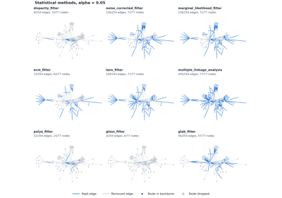
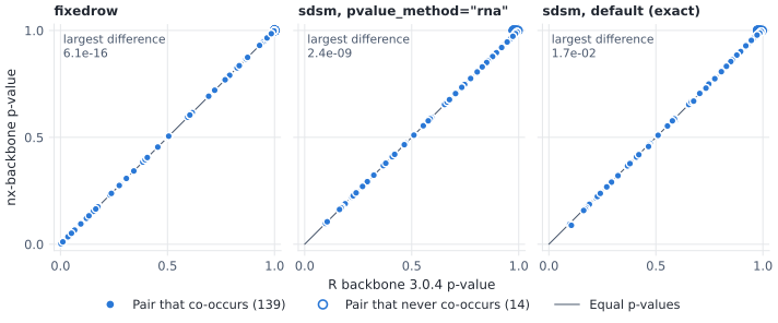
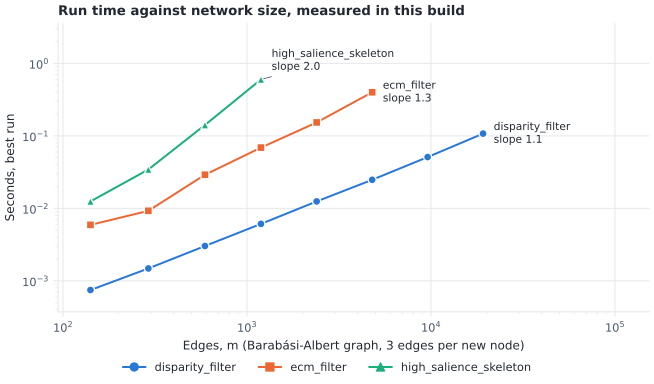
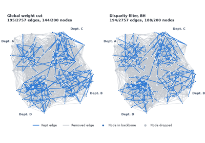
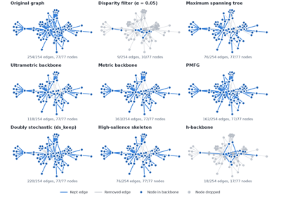
Method gallery
global_threshold_filter() on Les Misérables, keeping global_threshold_keep (threshold=2.0).
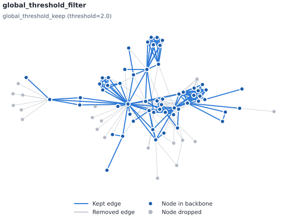
Backbone (blue) over the original graph (gray). Kept 157 of 254 edges (62%) and 58 of 77 nodes.#
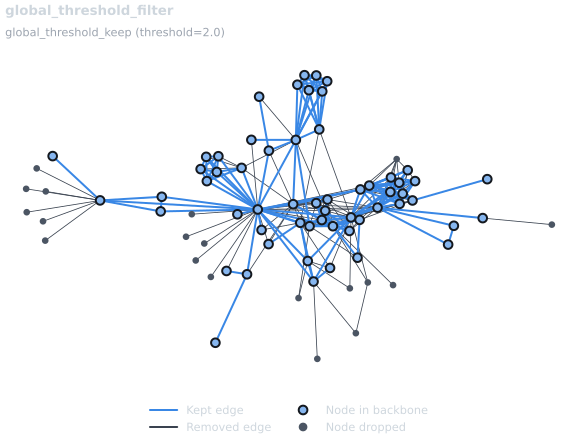
Backbone (blue) over the original graph (gray). Kept 157 of 254 edges (62%) and 58 of 77 nodes.#
strongest_n_ties() on Les Misérables, keeping strongest_n_ties_keep (n=2).
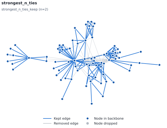
Backbone (blue) over the original graph (gray). Kept 146 of 254 edges (57%) and 77 of 77 nodes.#
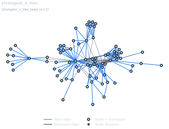
Backbone (blue) over the original graph (gray). Kept 146 of 254 edges (57%) and 77 of 77 nodes.#
global_sparsification() on Les Misérables, keeping global_sparsification_keep (s=0.4).
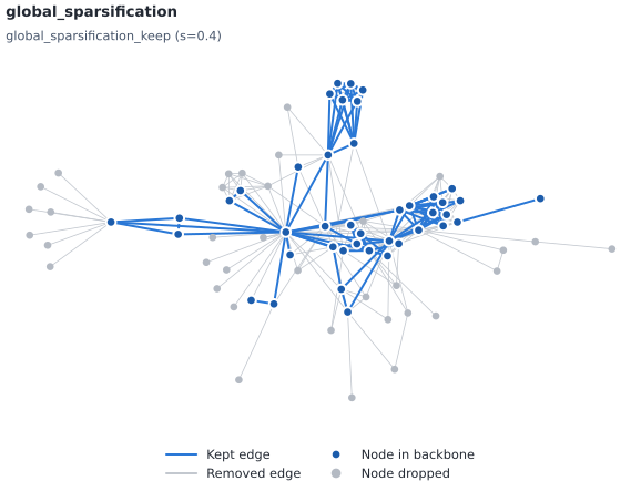
Backbone (blue) over the original graph (gray). Kept 102 of 254 edges (40%) and 42 of 77 nodes.#
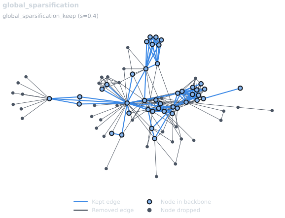
Backbone (blue) over the original graph (gray). Kept 102 of 254 edges (40%) and 42 of 77 nodes.#
primary_linkage_analysis() on Les Misérables, keeping primary_linkage_keep.
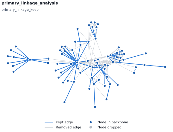
Backbone (blue) over the original graph (gray). Kept 69 of 254 edges (27%) and 77 of 77 nodes.#
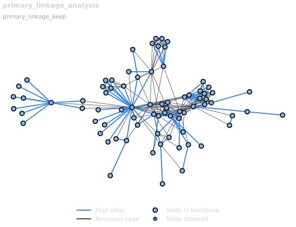
Backbone (blue) over the original graph (gray). Kept 69 of 254 edges (27%) and 77 of 77 nodes.#
edge_betweenness_filter() on Les Misérables, keeping edge_betweenness_keep (s=0.3).
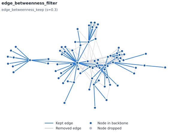
Backbone (blue) over the original graph (gray). Kept 77 of 254 edges (30%) and 77 of 77 nodes.#
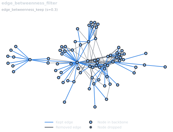
Backbone (blue) over the original graph (gray). Kept 77 of 254 edges (30%) and 77 of 77 nodes.#
node_degree_filter() on Les Misérables, keeping node_degree_keep (min_degree=2).
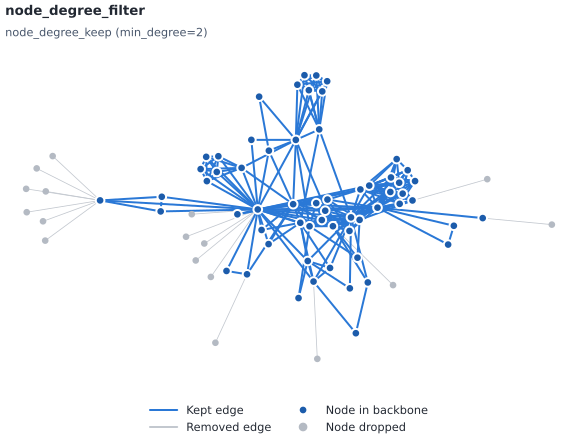
Backbone (blue) over the original graph (gray). Kept 237 of 254 edges (93%) and 60 of 77 nodes.#
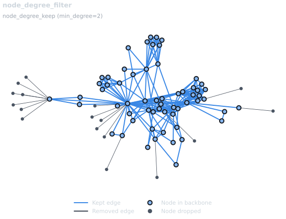
Backbone (blue) over the original graph (gray). Kept 237 of 254 edges (93%) and 60 of 77 nodes.#
high_salience_skeleton() on Les Misérables, keeping salience ≥ 0.5.
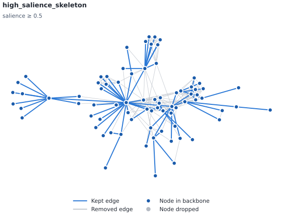
Backbone (blue) over the original graph (gray). Kept 76 of 254 edges (30%) and 77 of 77 nodes.#
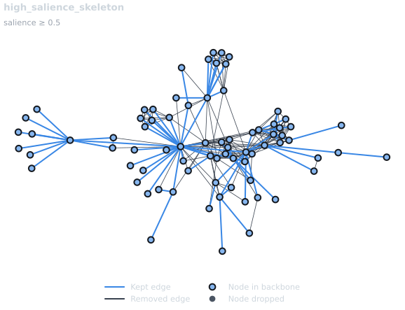
Backbone (blue) over the original graph (gray). Kept 76 of 254 edges (30%) and 77 of 77 nodes.#
metric_backbone() on Les Misérables, keeping metric_keep.
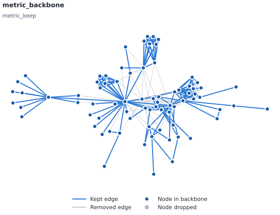
Backbone (blue) over the original graph (gray). Kept 163 of 254 edges (64%) and 77 of 77 nodes.#
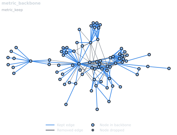
Backbone (blue) over the original graph (gray). Kept 163 of 254 edges (64%) and 77 of 77 nodes.#
ultrametric_backbone() on Les Misérables, keeping ultrametric_keep.
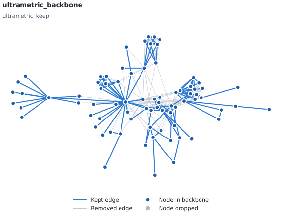
Backbone (blue) over the original graph (gray). Kept 118 of 254 edges (46%) and 77 of 77 nodes.#
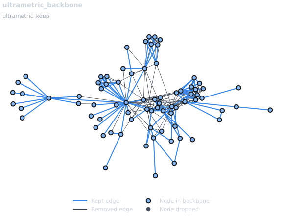
Backbone (blue) over the original graph (gray). Kept 118 of 254 edges (46%) and 77 of 77 nodes.#
doubly_stochastic_filter() on Les Misérables, keeping ds_weight ≥ 0.1.
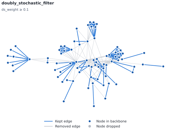
Backbone (blue) over the original graph (gray). Kept 109 of 254 edges (43%) and 77 of 77 nodes.#
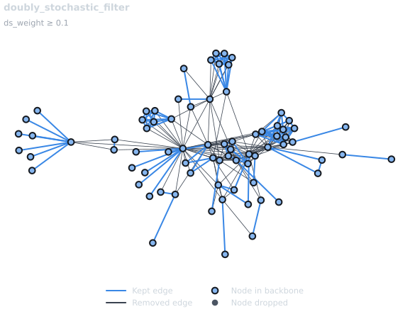
Backbone (blue) over the original graph (gray). Kept 109 of 254 edges (43%) and 77 of 77 nodes.#
h_backbone() on Les Misérables, keeping h_backbone_keep.
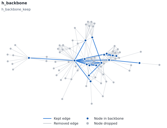
Backbone (blue) over the original graph (gray). Kept 18 of 254 edges (7%) and 17 of 77 nodes.#
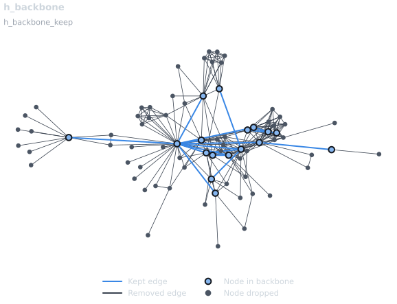
Backbone (blue) over the original graph (gray). Kept 18 of 254 edges (7%) and 17 of 77 nodes.#
modularity_backbone() on Les Misérables, keeping modularity_keep (seed=42).
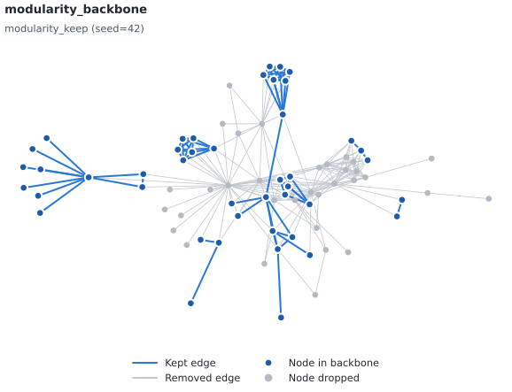
Backbone (blue) over the original graph (gray). Kept 72 of 254 edges (28%) and 44 of 77 nodes.#
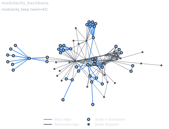
Backbone (blue) over the original graph (gray). Kept 72 of 254 edges (28%) and 44 of 77 nodes.#
planar_maximally_filtered_graph() on Les Misérables, keeping pmfg_keep.
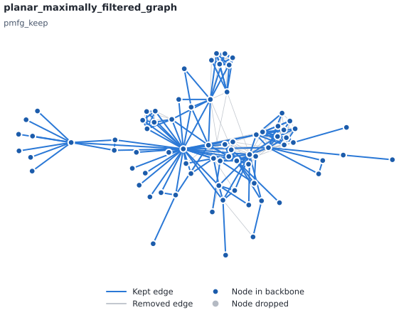
Backbone (blue) over the original graph (gray). Kept 162 of 254 edges (64%) and 77 of 77 nodes.#
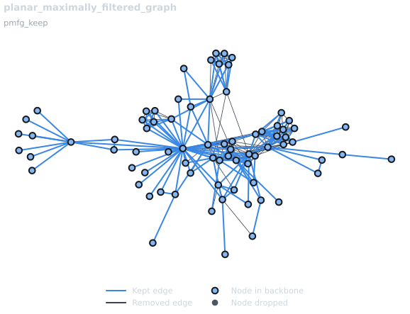
Backbone (blue) over the original graph (gray). Kept 162 of 254 edges (64%) and 77 of 77 nodes.#
maximum_spanning_tree_backbone() on Les Misérables, keeping mst_keep.
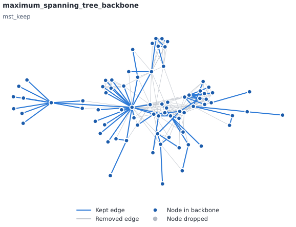
Backbone (blue) over the original graph (gray). Kept 76 of 254 edges (30%) and 77 of 77 nodes.#
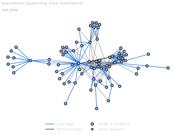
Backbone (blue) over the original graph (gray). Kept 76 of 254 edges (30%) and 77 of 77 nodes.#