Note
Go to the end to download the full example code.
Statistical null models side by side#
Every statistical backbone method asks the same question of each edge: is this edge heavier than chance would make it? The answer depends entirely on what “chance” means. A null model is that definition: a description of how the weights would be spread if nothing interesting were going on. An edge whose weight would be very unlikely under the null model gets a small p-value and is kept in the backbone, the sparse subgraph of edges that survive.
nx-backbone has seven statistical scorers, and each one encodes a different idea of chance. This tutorial runs all seven on the same graph and looks at what that choice does:
what each null model holds fixed;
whether a method does more than keep the heaviest edges;
which backbones contain which;
what each backbone preserves of the original network;
how to loosen or adjust a null model (
a=,unit=andtransform_weights());edges that are significantly weak, and how ties are signed.
Every number below is computed when the documentation is built. For the calls themselves, method by method, see the short how-to tutorial Statistical Backbone Extraction.
The network#
We use the Les Misérables co-appearance network that ships with NetworkX: 77 characters, linked when they appear together, with an integer weight that counts how often they do. It is small enough to draw, and its weights are genuine counts, which some of the null models need.
A node’s degree is its number of links and its strength is the sum of their weights. We use a significance level (alpha) of 0.05 throughout, without a multiple-testing correction, so that the backbones are comparable with the uncorrected comparison of Yassin et al. (2025). Validating a Backbone shows how a correction changes them.
import math
import warnings
from itertools import pairwise
from pathlib import Path

import matplotlib.pyplot as plt
import networkx as nx
import numpy as np
from _figures import style
from matplotlib.lines import Line2D
from matplotlib.ticker import NullLocator
from scipy.stats import spearmanr

import nx_backbone as nb


G = nx.les_miserables_graph()
ALPHA = 0.05
print(
    f"{G.number_of_nodes()} nodes, {G.number_of_edges()} edges, "
    f"weights from {min(w for *_, w in G.edges(data='weight'))} "
    f"to {max(w for *_, w in G.edges(data='weight'))}"
)
77 nodes, 254 edges, weights from 1 to 31
One question, seven nulls#
The seven scorers differ in what they hold fixed when they imagine “no structure”. A local null model judges an edge from the point of view of one endpoint at a time; a global one compares it with the whole network; the rest look at both endpoints at once.
Method |
The null model, in one sentence |
Conditions on |
|---|---|---|
|
Each node splits its strength over its links at random, every share equally likely. |
Each endpoint’s strength and degree, one endpoint at a time (local). |
|
Each node hands out its strength one unit at a time through a self-reinforcing urn, so weight attracts more weight. |
Each endpoint’s strength and degree (local), plus one reinforcement parameter for the whole network. |
|
The links stay where they are and every link draws its weight from the network’s own weight distribution. |
The global weight distribution, and both endpoints’ degree and strength. |
|
Weights are noisy counts, and a pair’s expected weight grows with both endpoints’ strengths. |
Both endpoints’ strengths jointly, and the total weight. |
|
Every unit of weight picks its two endpoints at random, in proportion to their strengths. |
Both endpoints’ strengths jointly, and the total weight. |
|
The most random (maximum-entropy) integer-weighted graph whose expected degrees and strengths match the observed ones. |
Every node’s degree and strength at once. |
|
No parametric model: an edge is compared with the other weights of the same node. |
The empirical distribution (empirical CDF) of each endpoint’s weights. |
The formulas are in each function’s API page. One detail matters for everything below: the disparity, Pólya and LANS filters test an edge from each endpoint and keep the smaller p-value, so an edge needs to stand out at only one of its ends. (That makes them reject more often than alpha even when their null model is true; see Weights, Units, and Transforms.)
Every scorer returns a copy of the graph with a p-value on each edge, and
threshold_filter() keeps the edges below alpha.
METHODS = {
    "Disparity": (nb.disparity_filter, "disparity_pvalue"),
    "Pólya": (nb.polya_filter, "polya_pvalue"),
    "GloSS": (nb.gloss_filter, "gloss_pvalue"),
    "Noise-corrected": (nb.noise_corrected_filter, "nc_pvalue"),
    "MLF": (nb.marginal_likelihood_filter, "ml_pvalue"),
    "ECM": (nb.ecm_filter, "ecm_pvalue"),
    "LANS": (nb.lans_filter, "lans_pvalue"),
}

scored = {name: score(G) for name, (score, _) in METHODS.items()}
backbones = {
    name: nb.threshold_filter(scored[name], attr, ALPHA, include_all_nodes=False)
    for name, (_, attr) in METHODS.items()
}


def table(header, rows):
    """Print rows as an aligned plain-text table."""
    rows = [[str(c) for c in row] for row in [header, *rows]]
    widths = [max(len(r[i]) for r in rows) for i in range(len(header))]
    for k, row in enumerate(rows):
        print("  ".join(c.ljust(w) for c, w in zip(row, widths)).rstrip())
        if k == 0:
            print("  ".join("-" * w for w in widths))


table(
    ["Method", "Edges kept", "Nodes kept"],
    [
        [name, bb.number_of_edges(), bb.number_of_nodes()]
        for name, bb in backbones.items()
    ],
)
Method           Edges kept  Nodes kept
---------------  ----------  ----------
Disparity        9           10
Pólya            12          14
GloSS            3           6
Noise-corrected  126         71
MLF              126         71
ECM              72          63
LANS             109         77
Same question, very different answers: the strictest backbone keeps a
handful of edges and the most permissive keeps about half of the network.
Two of them coincide. The noise-corrected and marginal likelihood filters
test a weight against the same binomial null model, in which every unit
of weight picks a pair in proportion to both endpoints’ strengths; they
count an undirected pair slightly differently, and on this network they
keep the same edges. (The noise-corrected filter adds a score and its
standard deviation, which the paper thresholds with a rule that keeps far
more edges; see the Notes of
noise_corrected_filter() for why its default
p-value is the binomial one.) The figure puts every backbone on the same
layout, so the eye can compare them.
def draw_overview(mode):
    p = style.palette(mode)
    pos = style.layout(G, "les_miserables")
    fig, axes = plt.subplots(2, 4, figsize=(9.6, 5.6))
    for ax, name in zip(axes.flat, METHODS):
        counts = style.draw_backbone(
            ax, G, backbones[name], pos, mode=mode, legend=False, title=name
        )
        ax.text(
            0.0,
            -0.02,
            counts.short,
            transform=ax.transAxes,
            va="top",
            color=p.muted,
            fontsize=8,
        )
    key = axes.flat[-1]
    key.set_axis_off()
    key.legend(handles=style.legend_handles(mode), loc="center left")
    fig.tight_layout()
    return fig


save("nulls_overview", draw_overview)
save("nulls_overview", draw_overview, fmt="png", modes=("light",))  # thumbnail
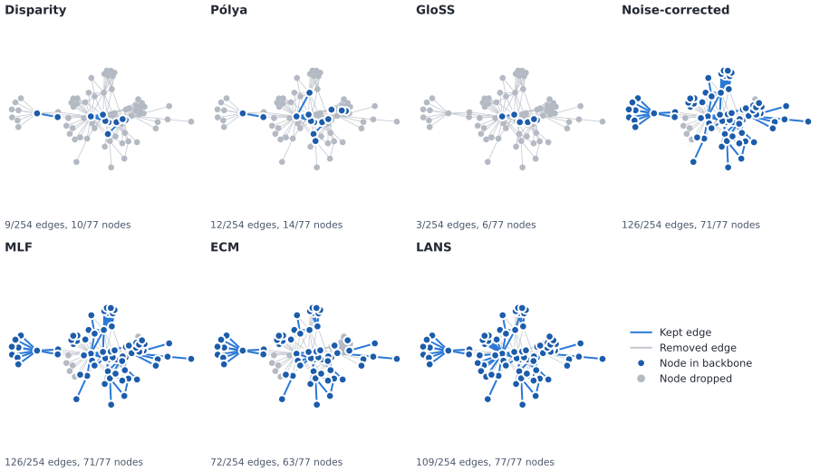
The seven backbones at alpha = 0.05, drawn over the original network (kept edges solid, removed edges faint; counts under each panel).#
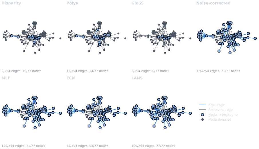
The seven backbones at alpha = 0.05, drawn over the original network (kept edges solid, removed edges faint; counts under each panel).#
P-value against weight#
The simplest backbone of all is a global weight threshold: keep every edge heavier than some cut-off. A statistical method is worth its extra assumptions only if it does something else, for example keeping a light edge of a node that has little weight to give, or dropping a heavy edge between two hubs that would be heavy anyway.
One way to see this is to plot each edge’s p-value against its weight, and to summarize the relation with Spearman’s rank correlation (rho), which is -1 when the p-value falls whenever the weight rises. Yassin et al. (2025) made the same comparison over 27 real networks.
weights = np.array([w for *_, w in G.edges(data="weight")], dtype=float)
pvals = {
    name: np.array([scored[name][u][v][attr] for u, v in G.edges()])
    for name, (_, attr) in METHODS.items()
}
rho = {name: spearmanr(weights, pv).statistic for name, pv in pvals.items()}
table(
    ["Method", "Spearman rho (p-value vs weight)"],
    [[name, f"{rho[name]:+.2f}"] for name in sorted(rho, key=rho.get)],
)
Method           Spearman rho (p-value vs weight)
---------------  --------------------------------
Pólya            -0.90
GloSS            -0.86
Disparity        -0.85
MLF              -0.63
Noise-corrected  -0.63
LANS             -0.38
ECM              -0.27
The weights are small integers, so the points are jittered a little to the left and right. P-values below one in a million are drawn at the bottom edge.
P_FLOOR = 1e-6
jitter = weights * np.exp(np.random.default_rng(0).uniform(-0.08, 0.08, weights.size))


def draw_scatter(mode):
    p = style.palette(mode)
    fig, axes = plt.subplots(2, 4, figsize=(9.6, 5.4), sharex=True, sharey=True)
    for ax, name in zip(axes.flat, METHODS):
        pv = np.clip(pvals[name], P_FLOOR, 1.0)
        kept = pvals[name] < ALPHA
        ax.scatter(
            jitter[~kept],
            pv[~kept],
            s=14,
            facecolors="none",
            edgecolors=p.muted,
            linewidths=0.6,
            alpha=0.7,
        )
        ax.scatter(
            jitter[kept], pv[kept], s=18, c=p.kept, edgecolors=p.surface, linewidths=0.5
        )
        ax.axhline(ALPHA, color=p.ink, lw=0.75, ls=(0, (3, 2)))
        ax.set_xscale("log")
        ax.set_yscale("log")
        ax.set_title(name)
        ax.text(
            1.0,
            1.0,
            f"rho = {rho[name]:+.2f}",
            transform=ax.transAxes,
            ha="right",
            va="bottom",
            color=p.muted,
            fontsize=8.5,
        )
        ax.grid(True)
    for ax in axes.flat:
        ax.xaxis.set_minor_locator(NullLocator())
        ax.yaxis.set_minor_locator(NullLocator())
    axes[0, 0].set_ylim(P_FLOOR / 3, 3)
    axes[0, 0].set_yticks([1e-6, 1e-4, 1e-2, 1], ["≤1e-6", "1e-4", "0.01", "1"])
    axes[0, 0].set_xticks([1, 3, 10, 30], ["1", "3", "10", "30"])
    key = axes.flat[-1]
    key.set_axis_off()
    key.legend(
        handles=[
            Line2D(
                [],
                [],
                marker="o",
                ls="",
                color=p.kept,
                markeredgecolor=p.surface,
                label="Kept (p < 0.05)",
            ),
            Line2D(
                [],
                [],
                marker="o",
                ls="",
                markerfacecolor="none",
                markeredgecolor=p.muted,
                label="Removed",
            ),
            Line2D([], [], color=p.ink, lw=0.75, ls=(0, (3, 2)), label="alpha = 0.05"),
        ],
        loc="center left",
    )
    fig.supxlabel("Edge weight (co-appearances, log scale)", fontsize=9)
    fig.supylabel("p-value (log scale)", fontsize=9)
    fig.tight_layout()
    return fig


save("nulls_pvalue_weight", draw_scatter)
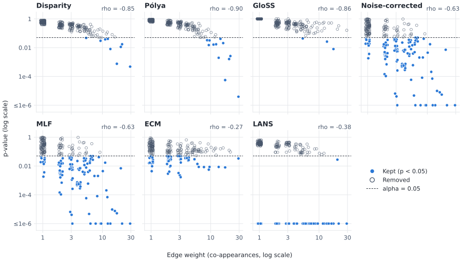
Each edge’s p-value against its weight. Filled dots are kept, hollow circles removed; rho is the Spearman rank correlation printed above.#
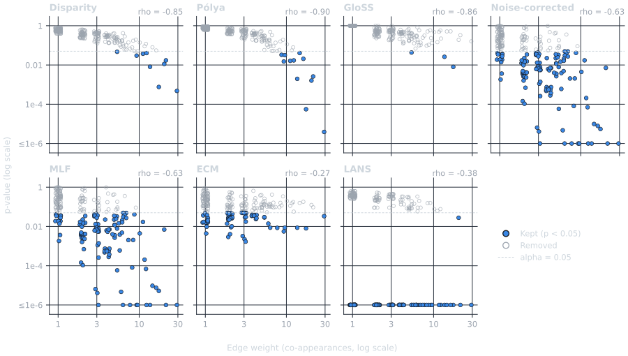
Each edge’s p-value against its weight. Filled dots are kept, hollow circles removed; rho is the Spearman rank correlation printed above.#
Three groups appear. The disparity, Pólya and GloSS p-values fall almost in lockstep with the weight: on this network they behave much like a weight threshold, with the cut-off set by each node’s share or by the global weight distribution. The ECM and LANS p-values are only loosely tied to the weight: those methods keep many light edges and drop some heavy ones, because they judge a weight against what the endpoints’ degrees and strengths (or the node’s other weights) lead one to expect. The noise-corrected and marginal likelihood p-values sit in between: they also judge a weight against its endpoints’ strengths, yet the heaviest edges still tend to be the most significant.
This is one network. Yassin et al. (2025) report that, across their 27 networks, the Pólya filter’s p-values are nearly uncorrelated with weight; on Les Misérables they are not. Averages over many networks are a guide, not a guarantee: check your own data.
Nestedness and overlap#
Do the methods find different edges, or the same edges with a stricter or looser bar? The overlap of backbone A with backbone B is the share of A’s edges that B also keeps. It is 1 when A is nested inside B, and it is not symmetric: a small backbone can sit entirely inside a large one but not the other way round.
order = sorted(METHODS, key=lambda name: backbones[name].number_of_edges())
edge_sets = {name: {frozenset(e) for e in backbones[name].edges()} for name in METHODS}
overlap = np.array(
    [
        [len(edge_sets[a] & edge_sets[b]) / max(len(edge_sets[a]), 1) for b in order]
        for a in order
    ]
)


def draw_overlap(mode):
    p = style.palette(mode)
    fig, ax = plt.subplots(figsize=(7.0, 5.4))
    im = ax.imshow(overlap, cmap=style.sequential_cmap(mode), vmin=0, vmax=1)
    for i in range(len(order)):
        for j in range(len(order)):
            value = overlap[i, j]
            ax.text(
                j,
                i,
                f"{value:.2f}",
                ha="center",
                va="center",
                fontsize=8.5,
                color=p.surface if value >= 0.5 else p.ink,
            )
    ax.set_xticks(range(len(order)), order, rotation=30, ha="right")
    ax.set_yticks(
        range(len(order)),
        [f"{name} ({len(edge_sets[name])})" for name in order],
    )
    ax.tick_params(length=0)
    for spine in ax.spines.values():
        spine.set_visible(False)
    ax.set_ylabel("Backbone A (edges kept)")
    ax.set_xlabel("Backbone B")
    ax.set_title("Share of A's edges that B also keeps")
    bar = fig.colorbar(im, ax=ax, fraction=0.046, pad=0.03)
    bar.outline.set_visible(False)
    bar.ax.tick_params(length=0)
    fig.tight_layout()
    return fig


save("nulls_overlap", draw_overlap)
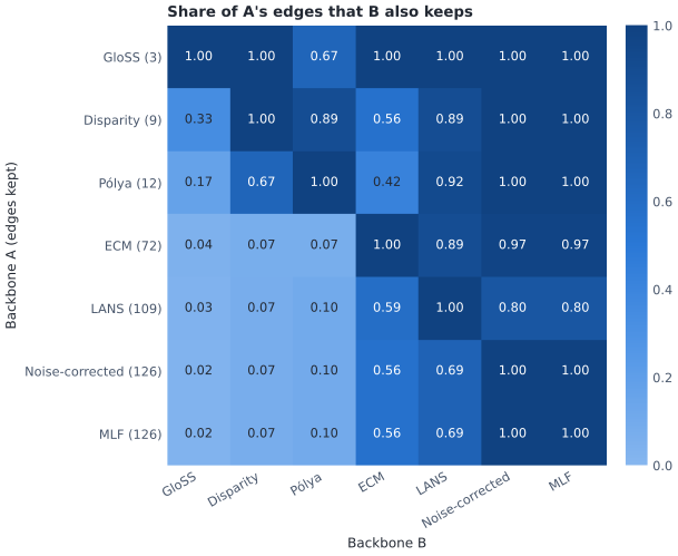
Overlap between backbones, smallest backbone first. Read along a row: the share of that backbone’s edges found in each other backbone.#
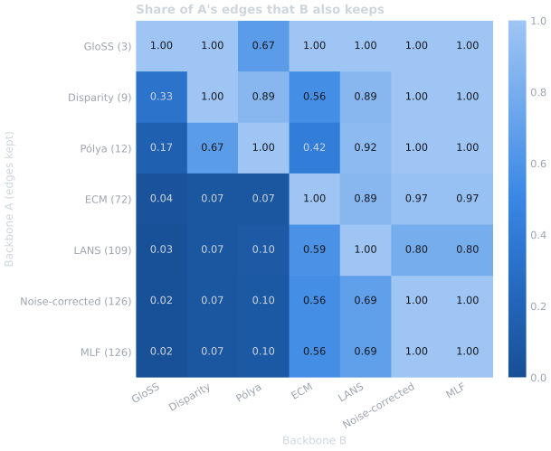
Overlap between backbones, smallest backbone first. Read along a row: the share of that backbone’s edges found in each other backbone.#
The three small backbones (GloSS, disparity and Pólya) lie entirely inside the noise-corrected and marginal likelihood backbones: on this network those methods agree on the strongest ties and differ in how far beyond them they go.
Yassin et al. (2025) found a hierarchy of this kind across their networks without correction, “GloSS ⊂ NC ⊂ PF ⊂ LANS ⊂ MLF”, with mean overlaps of 76%, 91%, 95% and 92% along the chain (their Fig 4). Here is the same chain on Les Misérables:
PAPER_CHAIN = [  # Yassin et al. (2025), Fig 4 text, no correction
    ("GloSS", "Noise-corrected", 0.76),
    ("Noise-corrected", "Pólya", 0.91),
    ("Pólya", "LANS", 0.95),
    ("LANS", "MLF", 0.92),
]
table(
    ["A", "B", "Overlap of A in B here", "Mean in Yassin et al."],
    [
        [a, b, f"{overlap[order.index(a), order.index(b)]:.2f}", f"{paper:.2f}"]
        for a, b, paper in PAPER_CHAIN
    ],
)
A                B                Overlap of A in B here  Mean in Yassin et al.
---------------  ---------------  ----------------------  ---------------------
GloSS            Noise-corrected  1.00                    0.76
Noise-corrected  Pólya            0.10                    0.91
Pólya            LANS             0.92                    0.95
LANS             MLF              0.80                    0.92
The chain breaks at its second link: the noise-corrected backbone is far
larger than the Pólya backbone here, so most of its edges cannot be in it.
The p-value is not the reason: like Yassin et al., who used the binomial
p-value of Coscia and Neffke (2017),
noise_corrected_filter() uses a binomial
p-value by default (the implementation they used counts the trials and
the tail slightly differently; see its Notes). A mean over 27 networks
says little about any one of them. Treat published hierarchies as
hypotheses to check, which takes one line with Python sets.
What each backbone preserves#
A backbone is a summary, and summaries distort. Two questions are
especially useful. Does the backbone keep the original weight
distribution, or only its heavy tail? And does it keep the degree
distribution, or only the hubs? The two-sample Kolmogorov-Smirnov
(KS) distance measures each: the largest gap between the two cumulative
distributions, from 0 (identical) to 1 (no overlap).
ks_weight() and
ks_degree() compute them. The degrees here are
those of the nodes each backbone keeps (include_all_nodes=False), so
dropped nodes do not count as degree 0.
preserved = {
    name: {
        "edges": nb.edge_fraction(G, bb),
        "weight": nb.weight_fraction(G, bb),
        "ks_weight": nb.ks_weight(G, bb),
        "ks_degree": nb.ks_degree(G, bb),
    }
    for name, bb in backbones.items()
}
table(
    ["Method", "Edge share", "Weight share", "KS weights", "KS degrees"],
    [
        [
            name,
            f"{m['edges']:.2f}",
            f"{m['weight']:.2f}",
            f"{m['ks_weight']:.2f}",
            f"{m['ks_degree']:.2f}",
        ]
        for name, m in ((n, preserved[n]) for n in order)
    ],
)


PANELS = [
    ("edges", "Share of edges kept"),
    ("ks_weight", "KS distance, weights"),
    ("ks_degree", "KS distance, degrees"),
]


def draw_preserved(mode):
    p = style.palette(mode)
    fig, axes = plt.subplots(1, 3, figsize=(9.6, 3.4), sharey=True)
    y = np.arange(len(order))
    for ax, (key, title) in zip(axes, PANELS):
        values = [preserved[name][key] for name in order]
        ax.hlines(y, 0, values, color=p.removed, lw=1.0)
        ax.scatter(values, y, s=40, c=p.kept, edgecolors=p.surface, linewidths=1.0)
        ax.set_xlim(0, 1)
        ax.set_title(title)
        ax.grid(True, axis="x")
        ax.tick_params(axis="y", length=0)
    axes[0].set_yticks(y, order)
    axes[0].invert_yaxis()
    axes[1].set_xlabel("0 = same distribution as the original, 1 = no overlap")
    fig.tight_layout()
    return fig


save("nulls_preserved", draw_preserved)
Method           Edge share  Weight share  KS weights  KS degrees
---------------  ----------  ------------  ----------  ----------
GloSS            0.01        0.04          0.80        0.78
Disparity        0.04        0.17          0.84        0.53
Pólya            0.05        0.23          0.93        0.53
ECM              0.28        0.31          0.16        0.52
LANS             0.43        0.55          0.12        0.42
Noise-corrected  0.50        0.73          0.27        0.31
MLF              0.50        0.73          0.27        0.31
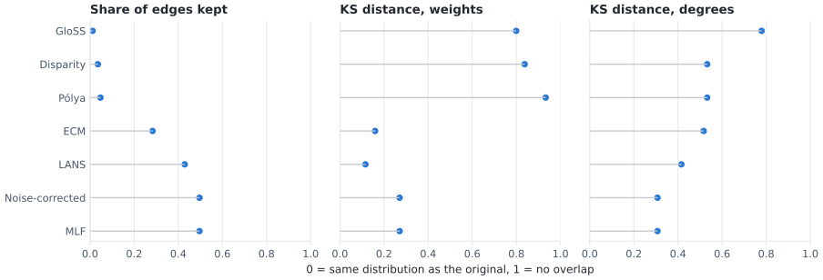
What each backbone keeps (left) and how far its weight and degree distributions move from the original’s (middle, right; lower is closer). The values are in the table above.#
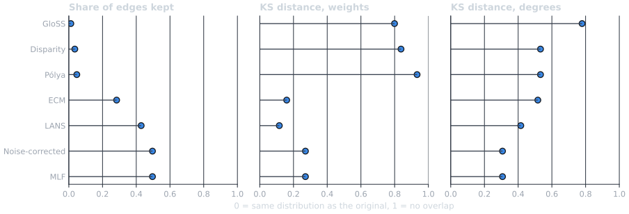
What each backbone keeps (left) and how far its weight and degree distributions move from the original’s (middle, right; lower is closer). The values are in the table above.#
Size explains part of this. The small backbones keep only heavy edges between a few characters, so both of their distributions move a long way, and the largest backbones (noise-corrected and marginal likelihood, which coincide here) keep the degree distribution best. But the ECM and LANS, with fewer edges, keep the weight distribution better than those two, because the edges they keep are lighter on average (their share of the weight is closer to their share of the edges). The ECM keeps the degree distribution worse than the marginal likelihood filter, though. Its null model already accounts for each node’s number of links, so the edges it keeps are the ones that degrees and strengths do not explain, and on this network they touch fewer nodes.
On so small a network the KS distance is coarse: Yassin et al. (2025) computed it only for networks with at least 1,000 edges. Read it as a description of this graph, not as a ranking of methods.
Loosening the null model#
A null model is an assumption, and some of these assumptions come with a dial. This section turns three of them.
The disparity filter’s concentration#
The disparity filter assumes that a node’s weight shares are as uneven as
random cut points make them. Real shares may be more even than that, or
more uneven. disparity_filter(G, a=...) makes the evenness a
parameter: a=1 is the original filter, a > 1 expects more uneven
shares (so fewer edges stand out), a < 1 more even ones. a="ml"
fits a to the network by maximum likelihood.
A_GRID = np.geomspace(0.1, 10, 25)
sweep = [
    nb.threshold_filter(
        nb.disparity_filter(G, a=a), "disparity_pvalue", ALPHA
    ).number_of_edges()
    for a in A_GRID
]
fitted = nb.disparity_filter(G, a="ml")
a_hat = fitted.graph["disparity_a"]
kept_fitted = nb.threshold_filter(fitted, "disparity_pvalue", ALPHA).number_of_edges()
print(f"Fitted a = {a_hat:.3f}: {kept_fitted} edges kept")
print(f"a = 1 (Serrano et al.): {backbones['Disparity'].number_of_edges()} edges kept")
print(f"Pólya filter's own fitted a: {scored['Pólya'].graph['polya_a']:.3f}")


def draw_concentration(mode):
    p = style.palette(mode)
    fig, ax = plt.subplots(figsize=(7.0, 3.4))
    ax.plot(A_GRID, sweep, color=p.kept, marker="o", markersize=4)
    marks = [
        (1.0, backbones["Disparity"].number_of_edges(), "a = 1, the original filter"),
        (a_hat, kept_fitted, f"fitted a = {a_hat:.2f}"),
    ]
    for a, kept, label in marks:
        ax.axvline(a, color=p.removed, lw=0.75)
        ax.scatter([a], [kept], s=60, c=p.node, edgecolors=p.surface, zorder=3)
        ax.annotate(
            f"{label}: {kept} edges",
            (a, kept),
            xytext=(8, 10),
            textcoords="offset points",
            color=p.ink,
            fontsize=8.5,
        )
    ax.set_xscale("log")
    ax.xaxis.set_minor_locator(NullLocator())
    ax.set_xticks([0.1, 0.3, 1, 3, 10], ["0.1", "0.3", "1", "3", "10"])
    ax.set_xlabel("Heterogeneity parameter a (log scale)")
    ax.set_ylabel(f"Edges kept at alpha = {ALPHA}")
    ax.set_title("Disparity filter backbone size as the null model loosens")
    ax.grid(True, axis="y")
    fig.tight_layout()
    return fig


save("nulls_disparity_a", draw_concentration)
Fitted a = 0.525: 19 edges kept
a = 1 (Serrano et al.): 9 edges kept
Pólya filter's own fitted a: 0.340
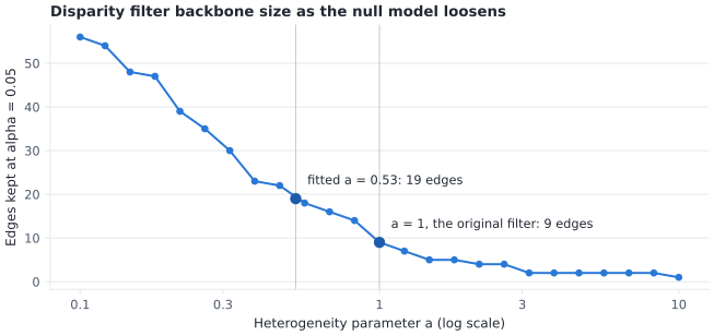
Disparity backbone size against a. The labeled points are the
original filter (a=1) and the maximum-likelihood fit.#
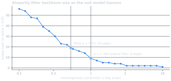
Disparity backbone size against a. The labeled points are the
original filter (a=1) and the maximum-likelihood fit.#
The fitted a is below 1: Les Misérables’ weight shares are more even than the original null model assumes, so an edge needs less of a node’s strength to stand out, and the fitted filter keeps more edges. The parameter means the same thing as the Pólya filter’s reinforcement parameter, but the two fits use different likelihoods (shares here, integer counts there), so their estimates differ. Whatever a you use, report it with the backbone.
Count units#
The marginal likelihood filter, the ECM and the noise-corrected filter
treat a weight as a number of events. More events is more evidence: a
share that could be a fluke over 3 events is convincing over 300. So
their p-values depend on the unit the weights are counted in, and the
unit= argument sets it: the models use weight / unit events. If
each co-appearance were really several events (several scenes, say), the
unit would be smaller than 1.
EVENTS = [1, 2, 4, 10]  # events per unit of weight, so unit = 1 / events
COUNT_MODELS = ["MLF", "ECM", "Noise-corrected"]
unit_sweep = {
    name: [
        nb.threshold_filter(
            METHODS[name][0](G, unit=1 / k), METHODS[name][1], ALPHA
        ).number_of_edges()
        for k in EVENTS
    ]
    for name in COUNT_MODELS
}
table(
    ["Method", *(f"unit=1/{k}" if k > 1 else "unit=1" for k in EVENTS)],
    [[name, *counts] for name, counts in unit_sweep.items()],
)


def draw_units(mode):
    p = style.palette(mode)
    colors = style.categorical(len(COUNT_MODELS), mode)
    fig, ax = plt.subplots(figsize=(7.0, 3.4))
    # Direct labels at the line ends, nudged apart where the lines end close.
    label_y, floor = {}, -math.inf
    for name in sorted(COUNT_MODELS, key=lambda n: unit_sweep[n][-1]):
        floor = max(unit_sweep[name][-1], floor + 16)
        label_y[name] = floor
    for name, color, marker in zip(COUNT_MODELS, colors, ["o", "s", "^"]):
        ax.plot(EVENTS, unit_sweep[name], color=color, marker=marker, label=name)
        ax.annotate(
            name,
            (EVENTS[-1], label_y[name]),
            xytext=(8, 0),
            textcoords="offset points",
            va="center",
            color=p.ink,
            fontsize=8.5,
        )
    ax.set_xscale("log")
    ax.xaxis.set_minor_locator(NullLocator())
    ax.set_xticks(EVENTS, [str(k) for k in EVENTS])
    ax.set_xlim(0.85, 22)
    ax.set_ylim(0, G.number_of_edges())
    ax.set_xlabel("Events per unit of weight (1 / unit, log scale)")
    ax.set_ylabel(f"Edges kept at alpha = {ALPHA}")
    ax.set_title("Count models keep more edges when a weight is more events")
    ax.grid(True, axis="y")
    ax.legend(loc="lower right")
    fig.tight_layout()
    return fig


save("nulls_units", draw_units)
Method           unit=1  unit=1/2  unit=1/4  unit=1/10
---------------  ------  --------  --------  ---------
MLF              126     165       194       215
ECM              72      79        83        89
Noise-corrected  126     165       194       215
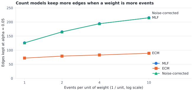
Edges kept by the three count models as each unit of weight counts as more events. The values are in the table above.#
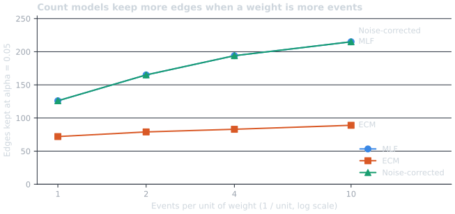
Edges kept by the three count models as each unit of weight counts as more events. The values are in the table above.#
The unit is part of the model, not a detail: if your weights are minutes, dollars or shares rather than counts, decide what one event is before you trust these three methods, and report it.
Transforming the weights#
transform_weights() returns a copy of the graph
with transformed weights, for example log(1 + w) to tame a heavy tail.
Which backbones does that change? It depends on what each method reads
from a weight: only the order of a node’s weights (LANS), a node’s shares
(disparity), or counts of events (the count models). We compare the
original weights, every weight times 4 (a change of scale), and
log(1 + w) (an increasing but nonlinear transform). The Pólya filter
is given its fitted a from the original weights, because its fit needs
integer weights.
a_polya = scored["Pólya"].graph["polya_a"]
VARIANTS = {
    "original": G,
    "4 w": nb.transform_weights(G, lambda w: 4 * w),
    "log(1 + w)": nb.transform_weights(G, math.log1p),
}


def backbone_of(name, H):
    score, attr = METHODS[name]
    scored_h = score(H, a=a_polya) if name == "Pólya" else score(H)
    return {frozenset(e) for e in nb.threshold_filter(scored_h, attr, ALPHA).edges()}


warned = set()
transformed = {}
for name in METHODS:
    for label, H in VARIANTS.items():
        with warnings.catch_warnings(record=True) as caught:
            warnings.simplefilter("always")
            transformed[name, label] = backbone_of(name, H)
        if caught:
            warned.add(name)

rows = []
for name in METHODS:
    base = transformed[name, "original"]
    cells = [
        f"{len(transformed[name, label])}"
        + ("" if transformed[name, label] == base else " (changed)")
        for label in VARIANTS
    ]
    rows.append([name, *cells])
table(["Method", *(f"edges, {label}" for label in VARIANTS)], rows)
print("\nWarned that log(1 + w) weights are not counts:", ", ".join(sorted(warned)))
Method           edges, original  edges, 4 w     edges, log(1 + w)
---------------  ---------------  -------------  -----------------
Disparity        9                9              0 (changed)
Pólya            12               22 (changed)   6 (changed)
GloSS            3                3              4 (changed)
Noise-corrected  126              194 (changed)  41 (changed)
MLF              126              194 (changed)  45 (changed)
ECM              72               83 (changed)   41 (changed)
LANS             109              109            109

Warned that log(1 + w) weights are not counts: ECM, MLF, Noise-corrected
Three behaviors, as the invariance table in Weights, Units, and Transforms predicts:
LANS uses only the order of each node’s weights, so neither transform changes it.
The disparity filter uses shares, which a change of scale leaves alone and
log(1 + w)does not. After the transform it tests whether the shares of the log-weights are even: a different hypothesis, which may be the one you want, but which should be reported as such.The count models change under both. Multiplying every weight by 4 is exactly the same as
unit=1/4above, and afterlog(1 + w)the weights are no longer counts at all, which is why those methods warn. Useunit=for a change of unit, and do not feed them transformed weights.The Pólya filter reads integer weights as urn draws, so it changes under both, like the count models. GloSS draws its null weights from the network’s own weights, so a change of scale moves the null with them;
log(1 + w)does not, because sums of log-weights behave differently from sums of weights.
Significantly weak edges#
The tests so far are one-sided: they only ask whether an edge is
stronger than expected. With signed=True, five of the scorers run a
two-sided test, and an edge can also be significantly weak: two
characters who appear together less often than their prominence predicts.
Each scored edge gets a sign attribute, +1 for strong and -1 for weak.
(The Pólya and GloSS filters define only the one-sided test.)
SIGNED = ["Disparity", "Noise-corrected", "MLF", "ECM", "LANS"]
signed = {name: METHODS[name][0](G, signed=True) for name in SIGNED}
signed_backbones = {
    name: nb.threshold_filter(
        signed[name], METHODS[name][1], ALPHA, include_all_nodes=False
    )
    for name in SIGNED
}


def sign_counts(H):
    signs = [s for *_, s in H.edges(data="sign")]
    return signs.count(1), signs.count(-1)


table(
    ["Method", "Strong (+1)", "Weak (-1)"],
    [[name, *sign_counts(bb)] for name, bb in signed_backbones.items()],
)


def draw_signed(mode):
    p = style.palette(mode)
    pos = style.layout(G, "les_miserables")
    fig, axes = plt.subplots(1, 2, figsize=(9.6, 4.9))
    for ax, name in zip(axes, ["MLF", "LANS"]):
        style.draw_backbone(
            ax,
            G,
            signed_backbones[name],
            pos,
            mode=mode,
            sign="sign",
            legend=False,
            title=f"{name}, signed",
        )
        plus, minus = sign_counts(signed_backbones[name])
        ax.text(
            0.0,
            -0.02,
            f"{plus} strong, {minus} weak",
            transform=ax.transAxes,
            va="top",
            color=p.muted,
            fontsize=8.5,
        )
    fig.legend(
        handles=style.legend_handles(mode, signed=True),
        loc="lower center",
        ncols=5,
        handlelength=2.4,
    )
    fig.tight_layout(rect=(0, 0.07, 1, 1))
    return fig


save("nulls_signed", draw_signed)
Method           Strong (+1)  Weak (-1)
---------------  -----------  ---------
Disparity        5            0
Noise-corrected  105          1
MLF              105          1
ECM              31           0
LANS             68           126
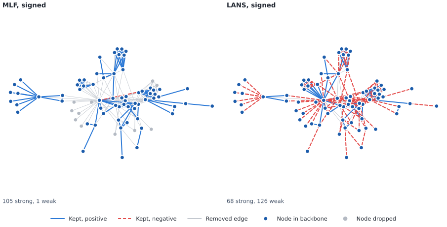
Signed backbones at alpha = 0.05: strong edges solid, weak edges dashed. The counts are in the table above.#
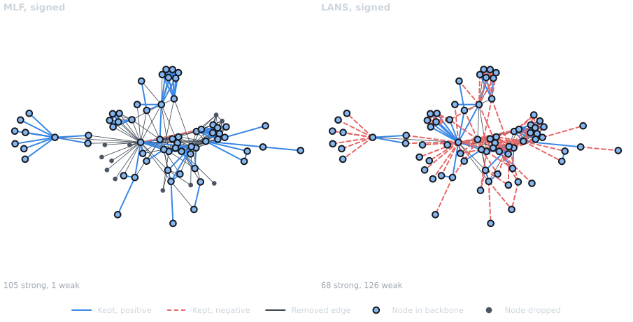
Signed backbones at alpha = 0.05: strong edges solid, weak edges dashed. The counts are in the table above.#
The parametric models rarely call an edge weak on this network: an edge can only be weak if the model expected it to be heavy, which needs two prominent endpoints. LANS calls many edges weak, because it is nonparametric: each node’s lightest link is as extreme, at the bottom, as its heaviest is at the top.
Ties, and the R convention#
Some links are both a node’s heaviest and its lightest. Napoleon appears with one character only, Myriel, so that single link is at once the top and the bottom of Napoleon’s weights. Under LANS its two tails are equal, and the test cannot say whether the link is strong or weak.
Napoleon's degree: 1
Signed LANS, Napoleon-Myriel: {'weight': 1, 'lans_pvalue': 0.0, 'sign': -1}
nx-backbone follows R backbone (Neal, 2022) here: an edge whose
two tails are exactly equal is signed -1. Neither choice is more correct;
matching R makes signed backbones directly comparable across the two
packages. The tie convention matters only when the two tails can be
equal, which for LANS happens often, at degree-1 nodes, at nodes whose
links all have the same weight, and on links that are the heaviest of one
endpoint and the lightest of the other.
Ties can be counted with the public API alone. The one-sided p-value is the upper tail, and the signed p-value is twice the smaller tail; so a weak edge whose one-sided p-value is half its signed p-value has equal tails.
one_sided = scored["LANS"]
weak = [
    (u, v) for u, v, d in signed_backbones["LANS"].edges(data=True) if d["sign"] == -1
]
ties = [
    (u, v)
    for u, v in weak
    if one_sided[u][v]["lans_pvalue"] == signed["LANS"][u][v]["lans_pvalue"] / 2
]
degree_one = [e for e in ties if min(G.degree(e[0]), G.degree(e[1])) == 1]
print(f"{len(weak)} weak LANS edges, {len(ties)} of them exact ties")
print(f"{len(degree_one)} of the ties have a degree-1 endpoint")
126 weak LANS edges, 40 of them exact ties
17 of the ties have a degree-1 endpoint
If your analysis reads the weak edges as evidence of avoidance, decide
what to do with the ties first: they say only that a node had too few, or
too similar, links to tell. The full comparison with R backbone and
netbone is in the design note on reference conventions in the
repository (docs/design/reference-conventions.md).
Choosing a null model deliberately#
Start from what a weight is. Counts of events suit the marginal likelihood filter, the ECM, the noise-corrected filter and the Pólya filter, with
unit=set to one event. Shares of a node’s activity suit the disparity filter. If only the order of the weights means anything, use LANS.Decide what “expected” should account for. Local methods ask whether a link matters to one of its nodes; the joint methods ask whether it is heavier than its two endpoints’ prominence explains; the ECM also accounts for every node’s number of links.
Check whether the method does more than threshold the weights on your data (the scatter above). If it does not, a global weight threshold is simpler to explain.
Report the null model’s settings (a,
unit=, any transform) and the significance level and correction, with the backbone.
Where next#
API pages: Statistical Methods (every scorer’s formulas and options), Filters (
threshold_filter(),transform_weights()) and Measures (the KS and fraction measures).User guide: Choosing a Method, Weights, Units, and Transforms and Evaluating Backbones.
Tutorials: Statistical Backbone Extraction (the calls, method by method), Validating a Backbone (multiple testing, robustness and signed backbones) and Comparing Multiple Methods.
References#
Coscia, M., & Neffke, F. M. (2017). Network backboning with noisy data. Proceedings of the IEEE International Conference on Data Engineering (ICDE), 425-436. https://doi.org/10.1109/ICDE.2017.100
Dianati, N. (2016). Unwinding the hairball graph: Pruning algorithms for weighted complex networks. Physical Review E, 93, 012304. https://doi.org/10.1103/PhysRevE.93.012304
Foti, N. J., Hughes, J. M., & Rockmore, D. N. (2011). Nonparametric sparsification of complex multiscale networks. PLoS ONE, 6(2), e16431. https://doi.org/10.1371/journal.pone.0016431
Gemmetto, V., Cardillo, A., & Garlaschelli, D. (2017). Irreducible network backbones: unbiased graph filtering via maximum entropy. arXiv:1706.00230.
Marcaccioli, R., & Livan, G. (2019). A Pólya urn approach to information filtering in complex networks. Nature Communications, 10, 745. https://doi.org/10.1038/s41467-019-08667-3
Neal, Z. P. (2022). backbone: An R package to extract network backbones. PLoS ONE, 17(5), e0269137. https://doi.org/10.1371/journal.pone.0269137
Radicchi, F., Ramasco, J. J., & Fortunato, S. (2011). Information filtering in complex weighted networks. Physical Review E, 83(4), 046101. https://doi.org/10.1103/PhysRevE.83.046101
Serrano, M. A., Boguñá, M., & Vespignani, A. (2009). Extracting the multiscale backbone of complex weighted networks. Proceedings of the National Academy of Sciences, 106(16), 6483-6488. https://doi.org/10.1073/pnas.0808904106
Yassin, A., Cherifi, H., Seba, H., & Togni, O. (2025). Backbone extraction through statistical edge filtering: A comparative study. PLoS ONE, 20(1), e0316141. https://doi.org/10.1371/journal.pone.0316141
Total running time of the script: (0 minutes 5.081 seconds)