Hypergraph backbones: keeping the groups that matter

Many social and biological records are lists of groups: who attended which meeting, which authors wrote which paper, which proteins form which complex. The usual first step turns every group into all of its pairs and analyzes the resulting graph. This tutorial is about the cases where that step throws away the thing you care about, and about the backbone methods that work on the groups directly.

We follow one small, real dataset from start to finish: the 18 women and 14 social events of Davis, Gardner & Gardner’s Deep South (1941), bundled with NetworkX as nx.davis_southern_women_graph(). Along the way we

1. compare a group view and a pairwise view of the same events;

2. extract the minimum description length (MDL) backbone of Kirkley, Felippe, Malizia & Battiston (2026) and look at the trade-off it optimizes;

3. run its local variant and see how its three aggregation rules differ;

4. switch to a synthetic meeting log to test which groups recur more often than chance, with the statistically validated hypergraphs and cores of Musciotto, Battiston & Mantegna (2021);

5. use the structural helpers (maximal hyperedges, order filtering, s-components); and

6. move hypergraphs in and out of the library with the HIF interchange format.

Every number on this page is computed when the documentation is built. The plotting code is left out of the page to keep the analysis readable; it is in the script and notebook you can download at the end. For a shorter, code-first reference to the same functions, see Hypergraph Backbones.

import base64
import html
import io
import itertools
import json
import math
import random
import re
import shutil
import tempfile
from pathlib import Path

import matplotlib.pyplot as plt
import networkx as nx
from _figures import style
from matplotlib.lines import Line2D
from matplotlib.ticker import MaxNLocator

import nx_backbone as nb

The data: women and the events they attended

A hypergraph is a set of nodes together with a set of hyperedges, where a hyperedge is any group of nodes, of any size. The size of a hyperedge is its order; an ordinary graph is a hypergraph whose hyperedges all have order two. NetworkX has no hypergraph class, so nx_backbone uses the simplest representation there is: a list of hyperedges, each an iterable of node labels.

In the Davis data each event is a hyperedge (the guest list) over the women. NetworkX ships the data as a bipartite graph, so the guest lists are the neighborhoods of the event nodes.

davis = nx.davis_southern_women_graph()
women = davis.graph["top"]
events = davis.graph["bottom"]
guest_lists = {event: frozenset(davis[event]) for event in events}
hyperedges = list(guest_lists.values())

# Two events can have identical guest lists.  The backbone functions merge
# such duplicates, so keep track of which events share one.
events_of = {}
for event, guests in guest_lists.items():
    events_of.setdefault(guests, []).append(event)
distinct = list(events_of)
label = {guests: "/".join(names) for guests, names in events_of.items()}

sizes = sorted(len(guests) for guests in hyperedges)
print(f"{len(women)} women, {len(events)} events, {len(distinct)} distinct guest lists")
print(f"event sizes (orders): {sizes}")
for guests, names in events_of.items():
    if len(names) > 1:
        print(f"{' and '.join(names)} had the same {len(guests)} guests")

18 women, 14 events, 13 distinct guest lists
event sizes (orders): [3, 3, 3, 3, 4, 4, 5, 6, 6, 8, 8, 10, 12, 14]
E13 and E14 had the same 3 guests

1. Groups versus pairs

The pairwise projection (or clique expansion) of a hypergraph links two nodes whenever they share at least one hyperedge. It is what you get when you analyze co-attendance as a graph of women. The projection is not reversible. A meeting of three people and three separate meetings of two produce exactly the same triangle:

one_meeting = [("A", "B", "C")]
three_meetings = [("A", "B"), ("B", "C"), ("A", "C")]


def projection(hyperedges):
    """The pairwise projection: one edge per pair of nodes sharing a hyperedge."""
    graph = nx.Graph()
    for members in hyperedges:
        graph.add_nodes_from(members)
        graph.add_edges_from(itertools.combinations(sorted(members), 2))
    return graph


same = nx.utils.edges_equal(
    projection(one_meeting).edges(), projection(three_meetings).edges()
)
print(f"Both hypergraphs project to the same triangle: {same}")

Both hypergraphs project to the same triangle: True

The incidence graph keeps the difference. It is a bipartite graph with one node per person, one node per hyperedge, and an edge for every membership; hypergraph_to_bipartite() builds it.

incidence_one, people = nb.hypergraph_to_bipartite(one_meeting)
incidence_three, _ = nb.hypergraph_to_bipartite(three_meetings)
for name, graph in [
    ("one meeting", incidence_one),
    ("three meetings", incidence_three),
]:
    print(
        f"{name}: {graph.number_of_nodes()} nodes "
        f"({len(people)} people), {graph.number_of_edges()} memberships"
    )

one meeting: 4 nodes (3 people), 3 memberships
three meetings: 6 nodes (3 people), 6 memberships

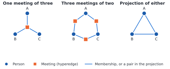
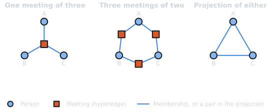
Figure 1. Two different hypergraphs, drawn as incidence graphs (people are circles, meetings are squares), have the same pairwise projection. The projection cannot tell a three-person meeting from three two-person meetings.

The same loss happens at scale. In the Davis data most pairs of women attended at least one event together, so the projection is close to a complete graph, and every pair of co-attendees looks alike whether they met at a small gathering or among a dozen other guests.

women_projection = projection(hyperedges)
print(
    f"incidence graph: {davis.number_of_nodes()} nodes, "
    f"{davis.number_of_edges()} memberships"
)
print(
    f"projection: {women_projection.number_of_nodes()} women, "
    f"{women_projection.number_of_edges()} pairs, "
    f"density {nx.density(women_projection):.2f}"
)

incidence graph: 32 nodes, 89 memberships
projection: 18 women, 139 pairs, density 0.91
Ignoring fixed y limits to fulfill fixed data aspect with adjustable data limits.
Ignoring fixed y limits to fulfill fixed data aspect with adjustable data limits.

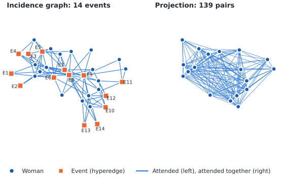
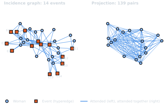
Figure 2. The Davis data as a hypergraph (left) and as its pairwise projection (right, density 0.91). Women keep their positions across the panels.

Pairwise backbones of the projection, such as the bipartite projection methods in Bipartite Projection Backbones, answer “which pairs are tied more than expected?”. The methods below answer a different question: “which groups do we need?”. Their output is a sub-hypergraph, a subset of the original hyperedges.

2. The MDL backbone

Look at the guest lists and you see redundancy: some small events are almost subsets of bigger ones. The MDL backbone of Kirkley, Felippe, Malizia & Battiston (2026) turns that observation into a compression problem. Imagine sending the hypergraph to someone, bit by bit. You choose a backbone of parent hyperedges, which you send in full. Every other hyperedge, a child, is sent as an edit of one parent it overlaps: say how many nodes they share, which ones, and which outside nodes complete the child. A child that nearly matches its parent is cheap to send.

The description length \(L(G, B)\) is the total number of bits needed for hypergraph \(G\) given backbone \(B\). It has two parts that pull against each other:

• the bits for the parents, which grow with every hyperedge kept, and

• the bits for the children given their parents, which grow as the backbone shrinks and children must be sent from poorer matches.

The MDL backbone is the \(B\) with the smallest total. The method has no parameters to tune on an unweighted hypergraph: the trade-off is decided by the bit counts alone.

result = nb.mdl_hypergraph_backbone(hyperedges)
print(f"kept {len(result.backbone)} of {result.n_input_hyperedges} distinct events")
for parent in result.backbone:
    children = result.assignment.get(parent, [])
    sent_from = ", ".join(label[c] for c in children) or "no children"
    print(f"  {label[parent]:>8} ({len(parent)} guests) encodes: {sent_from}")

kept 4 of 13 distinct events
        E3 (6 guests) encodes: E1, E2, E4, E5, E6, E9
        E7 (10 guests) encodes: no children
        E8 (14 guests) encodes: E11
       E10 (5 guests) encodes: E12, E13/E14

To see the trade-off, we can write the description length out ourselves. With \(N\) nodes and \(\ell\) distinct orders, a parent \(p\) costs \(\log_2 \ell + \log_2 \binom{N}{|p|}\) bits (its size, then which nodes), and a child \(c\) sent from parent \(p\), sharing \(o = |c \cap p|\) nodes, costs

\[\log_2 \ell + \log_2 \min(|c|, |p|) + \log_2 \binom{|p|}{o} + \log_2 \binom{N - |p|}{|c| - o}\]

bits: its size, the size of the overlap, which parent nodes are shared, and which outside nodes complete it. Each child goes to the overlapping parent that sends it most cheaply. The function below implements these two equations and checks itself against the library.

n_nodes, n_orders = result.n_nodes, result.n_orders


def parent_bits(parent):
    return math.log2(n_orders) + math.log2(math.comb(n_nodes, len(parent)))


def child_bits(child, parent):
    shared = len(child & parent)
    return (
        math.log2(n_orders)
        + math.log2(min(len(child), len(parent)))
        + math.log2(math.comb(len(parent), shared))
        + math.log2(math.comb(n_nodes - len(parent), len(child) - shared))
    )


def description_length(backbone):
    """(bits for the parents, bits for the children) of a candidate backbone."""
    backbone = set(backbone)
    parents = sum(parent_bits(p) for p in backbone)
    children = sum(
        min(child_bits(c, p) for p in backbone if c & p)
        for c in distinct
        if c not in backbone
    )
    return parents, children


print(f"library:   {result.description_length:.2f} bits")
print(f"by hand:   {sum(description_length(result.backbone)):.2f} bits")

library:   163.82 bits
by hand:   163.82 bits

Now compare backbones. Sending every event in full is one extreme: no children, but every bit is spent on parents. Keeping only the maximal events (those not contained in another event) is a purely structural reduction. At the other extreme, a greedy cover keeps the largest event and then only events that share no guest with what is already kept, which leaves almost everything to be sent as children.

Finding the exact optimum is a combinatorial search, so the library uses the two greedy optimizers of the paper’s Appendix D. method="edge" adds parent-child links in order of how many bits they save; method="node" adds parents in order of their total savings. method="auto" (the default, and what the paper does) runs both and keeps whichever gives the shorter description.

by_edge = nb.mdl_hypergraph_backbone(hyperedges, method="edge")
by_node = nb.mdl_hypergraph_backbone(hyperedges, method="node")

cover = []
for guests in sorted(distinct, key=len, reverse=True):
    if not any(guests & kept for kept in cover):
        cover.append(guests)

candidates = {
    "Every event": distinct,
    "Maximal events": nb.maximal_hyperedges(hyperedges),
    'MDL, method="edge"': by_edge.backbone,
    'MDL, method="node"': by_node.backbone,
    "Largest-first cover": cover,
}
baseline = result.baseline_description_length
print(
    f"{'backbone':<22}{'kept':>5}{'parents':>10}{'children':>10}{'total':>9}{'ratio':>7}"
)
for name, backbone in candidates.items():
    parents, children = description_length(backbone)
    total = parents + children
    print(
        f"{name:<22}{len(backbone):>5}{parents:>10.1f}{children:>10.1f}"
        f"{total:>9.1f}{total / baseline:>7.2f}"
    )
print(
    f'method="auto" kept {len(result.backbone)} events, {result.description_length:.1f} bits'
)

backbone               kept   parents  children    total  ratio
Every event              13     204.6       0.0    204.6   1.00
Maximal events            7     118.8      59.1    177.9   0.87
MDL, method="edge"        5      81.3      90.5    171.8   0.84
MDL, method="node"        4      66.2      97.6    163.8   0.80
Largest-first cover       1      14.6     199.5    214.1   1.05
method="auto" kept 4 events, 163.8 bits

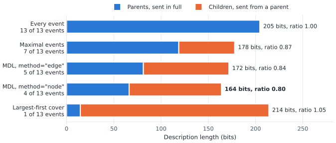
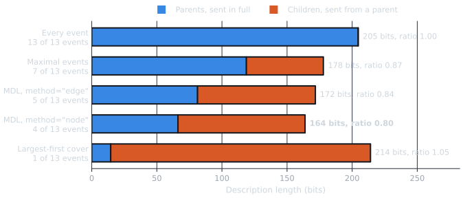
Figure 3. Description length of five candidate backbones of the Davis events. Keeping every event spends all bits on parents; the largest-first cover spends almost all of them on children. The shortest total (MDL, method="node", 164 bits) is the MDL backbone. The ratio is the total divided by the cost of sending every event in full; the table above gives the same values.

For the MDL backbone, the ratio in the last column is the paper’s inverse compression ratio \(\eta = L(G, B^*) / L(G, G)\): the description length of the MDL backbone divided by that of sending everything. It lies between 0 and 1. A value near 0 means the hypergraph is highly redundant; a value of 1 means no backbone shortens the description. A poor backbone can do worse than no backbone at all: the largest-first cover’s ratio is above 1. The MDL ratio is stored on the result, and hypergraph_compression_ratio() returns it directly.

print(f"eta = {result.compression_ratio:.3f}")
print(f"eta = {nb.hypergraph_compression_ratio(hyperedges):.3f}")

eta = 0.801
eta = 0.801

Figure 4 puts the MDL backbone back on the incidence graph. The kept events are the ones the others can be sent from cheaply; the pruned events are still in the data, encoded as edits of the kept ones (the printout above lists which parent encodes which child). The backbone holds guest lists, so map them back to the events:

kept_events = [e for e in events if guest_lists[e] in set(result.backbone)]
pruned_events = [e for e in events if e not in kept_events]
print(f"kept:   {', '.join(kept_events)}")
print(f"pruned: {', '.join(pruned_events)}")

kept:   E3, E7, E8, E10
pruned: E1, E2, E4, E5, E6, E9, E11, E12, E13, E14

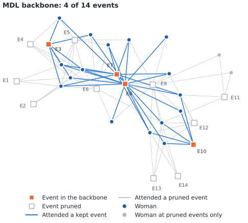
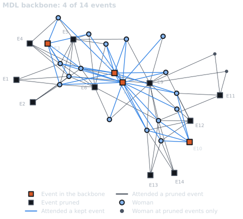
Figure 4. The MDL backbone of the Davis events. It keeps 4 of 14 events (counting both events of a shared guest list) and 35 of 89 memberships; 16 of 18 women attended at least one kept event.

Weighted hypergraphs. When hyperedges carry integer weights, such as how many times a group met, weights= and a single knob gamma in \((0, 1]\) let the weights pull heavy hyperedges into the backbone; gamma=1 ignores them. Hypergraph Backbones shows the call.

Reporting. describe_backbone() writes a methods paragraph with the citation, from the same reference list the library uses everywhere:

print(
    nb.describe_backbone(
        "mdl_hypergraph_backbone", original=hyperedges, backbone=result
    )
)

We extracted the backbone with the minimum description length (MDL) hypergraph backbone (Kirkley et al., 2026), which keeps the set of hyperedges from which the others can be encoded most cheaply, a parameter-free information-theoretic criterion. The backbone retains 4 of 13 distinct hyperedges (30.8%). Backbones were computed with nx-backbone version 0.3.0.post1.dev1 (Keegan, n.d.).

References

Keegan, B. C. (n.d.). nx-backbone: Backbone extraction algorithms for complex networks (Version 0.3.0.post1.dev1) [Python package]. https://github.com/brianckeegan/nx-backbone
Kirkley, A., Felippe, H., Malizia, F., & Battiston, F. (2026). Hypergraph backboning. arXiv:2606.00893.

3. The local MDL backbone

The MDL backbone is global: an event is pruned whenever any overlapping event, anywhere in the data, can send it cheaply. That can be unfair to a woman whose only events are pruned. The local variant (Appendix E of the paper) is the higher-order cousin of the disparity filter. Each woman’s neighborhood is the set of events she attended. The MDL backbone is found for every neighborhood on its own, so each woman “votes” for the events in her neighborhood backbone. An aggregation rule then decides how many votes an event needs:

• "union": at least one of its guests (every woman keeps at least one event, but the backbone is dense);

• "majority" (the default, used for Table II of the paper): at least half of its guests;

• "all": every guest (the most conservative rule).

local = {
    rule: nb.local_mdl_hypergraph_backbone(hyperedges, aggregation=rule)
    for rule in ("union", "majority", "all")
}
print(f"{'rule':<10}{'kept':>6}{'eta (local)':>13}")
print(f"{'global':<10}{len(result.backbone):>6}{result.compression_ratio:>13.3f}")
for rule, res in local.items():
    print(f"{rule:<10}{len(res.backbone):>6}{res.compression_ratio:>13.3f}")

rule        kept  eta (local)
global         4        0.801
union          8        0.880
majority       7        0.886
all            3        0.950

The per-woman results are on the result object. For example, the first woman’s neighborhood and its backbone:

first = women[0]
neighborhood = [label[g] for g in distinct if first in g]
own_backbone = [label[g] for g in local["majority"].local_backbones[first]]
print(
    f"{first} attended {len(neighborhood)} distinct events: {', '.join(neighborhood)}"
)
print(f"her neighborhood backbone keeps: {', '.join(own_backbone)}")
print(f"in {local['majority'].local_description_lengths[first]:.1f} bits")

Evelyn Jefferson attended 8 distinct events: E1, E2, E3, E4, E5, E6, E8, E9
her neighborhood backbone keeps: E3, E8
in 98.3 bits

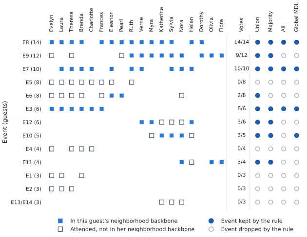
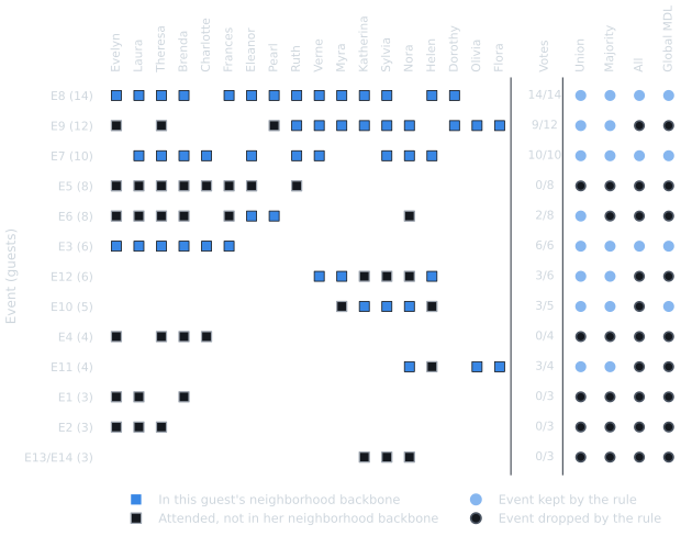
Figure 5. How the local MDL backbone votes. Each row is a guest list (events with identical lists are merged), each column a woman; filled squares are her votes. The union rule needs one vote, the majority rule needs votes from at least half of the guests, the all rule from every guest. Filled circles mark the events each rule keeps, next to the global MDL backbone for comparison.

Read Figure 5 row by row. An event that is the natural parent in many of its guests’ neighborhoods collects many votes; an event that sits almost inside a bigger one collects few or none, whatever its size. The global backbone (last column) can still drop an event that most of its guests vote for, when an event elsewhere sends it cheaply; the majority rule keeps such events. Choose the local backbone when each person’s important groups matter more than overall compression, and expect it to be denser and to compress less than the global one.

4. Statistically validated hypergraphs and cores

The MDL backbone asks which groups explain the structure. A different question is which groups recur more often than chance. That needs repeated observations, and in the Davis data no guest list repeats more than twice. So for this section we generate a synthetic meeting log: many small meetings drawn at random among colleagues, plus a few planted groups that meet again and again:

• a pair, a trio and a quartet, each meeting several times on their own;

• a trio that meets several times too, but every time with a different fourth colleague, so it never appears as a hyperedge by itself.

rng = random.Random(7)
colleagues = list(range(60))
meeting_log = [tuple(rng.sample(colleagues, rng.choice([2, 3, 4]))) for _ in range(600)]
planted = {(0, 1): 8, (2, 3, 4): 6, (5, 6, 7, 8): 5}
for group, times in planted.items():
    meeting_log += [group] * times
hidden_core = (9, 10, 11)
others = [c for c in colleagues if c not in hidden_core]
meeting_log += [(*hidden_core, rng.choice(others)) for _ in range(8)]
rng.shuffle(meeting_log)
print(f"{len(meeting_log)} meetings among {len(colleagues)} colleagues")

627 meetings among 60 colleagues

The statistically validated hypergraph (SVH) of Musciotto, Battiston & Mantegna (2021) tests every observed hyperedge against a null model, a random baseline that keeps how active each person is. Within each order \(k\), with \(n_k\) meetings of that size and \(d_i\) of them including person \(i\), the number of times a group meets is compared with a binomial distribution whose mean is \(n_k \prod_i (d_i / n_k)\). The p-value is the chance of seeing the group meet at least as often under that baseline. Because thousands of groups are tested, the p-values are controlled with the Benjamini-Hochberg false discovery rate (FDR) at level alpha, corrected for the number of possible groups of each order.

svh = nb.statistically_validated_hypergraph(meeting_log, alpha=0.01)


def expected_meetings(group, log):
    """Mean of the SVH null: n_k * prod(d_i / n_k) over meetings of size k."""
    same_order = [frozenset(m) for m in log if len(set(m)) == len(group)]
    n_k = len(same_order)
    expected = n_k
    for person in group:
        expected *= sum(person in m for m in same_order) / n_k
    return expected


print(f"validated {len(svh.validated)} of {len(svh.pvalues)} tested hyperedges")
print(f"{'group':<16}{'met':>5}{'expected':>10}{'p-value':>11}  validated")
for group in [*planted, hidden_core]:
    key = frozenset(group)
    if key in svh.pvalues:
        print(
            f"{group!s:<16}{svh.counts[key]:>5}{expected_meetings(group, meeting_log):>10.3f}"
            f"{svh.pvalues[key]:>11.1e}  {key in svh.validated}"
        )
    else:
        print(f"{group!s:<16}{0:>5}{'':>10}{'not tested':>11}  {key in svh.validated}")

validated 2 of 590 tested hyperedges
group             met  expected    p-value  validated
(0, 1)              8     1.189    3.2e-05  False
(2, 3, 4)           6     0.129    5.3e-09  True
(5, 6, 7, 8)        5     0.010    8.9e-13  True
(9, 10, 11)         0           not tested  False

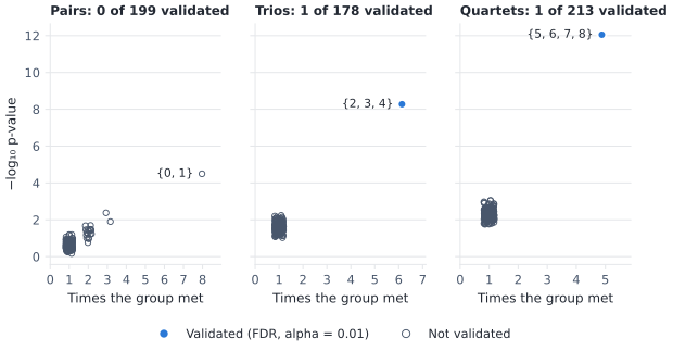
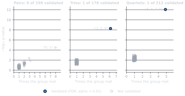
Figure 6. Every hyperedge of the meeting log tested by the SVH, one panel per order. Filled points are validated, hollow points are not; points are jittered horizontally so that groups with the same count do not hide each other. The planted groups are labeled.

The printout and Figure 6 show two things. First, repetition is judged relative to the order: a quartet that meets a few times is far more surprising than a pair that meets a few more times, because random pairs overlap often while random quartets almost never do (compare the expected counts in the table). Second, the trio that always came with a fourth person is invisible to the SVH, since it never appears as a hyperedge of its own.

The statistically validated cores (SVC) close that gap. They test every sub-group of every hyperedge, counting how many meetings contain it, from the largest order down; once a group is validated its subsets are not tested again, so significance goes to the largest validated core.

svc = nb.statistically_validated_cores(meeting_log, alpha=0.01)
print(f"tested {len(svc.pvalues)} groups, validated {len(svc.validated)} cores")
for core in svc.validated:
    alone = meeting_log.count(tuple(sorted(core)))
    print(
        f"  {sorted(core)!s:<14} in {svc.counts[core]} meetings "
        f"(alone in {alone}), p = {svc.pvalues[core]:.1e}"
    )

tested 2384 groups, validated 3 cores
  [5, 6, 7, 8]   in 5 meetings (alone in 5), p = 6.9e-14
  [2, 3, 4]      in 6 meetings (alone in 6), p = 3.9e-08
  [9, 10, 11]    in 8 meetings (alone in 0), p = 3.5e-12

The hidden trio is now found. SVC enumerates sub-groups, up to \(2^k\) for a hyperedge of size \(k\), so on data with large hyperedges set max_order (a guard, max_groups, stops runaway enumerations). Both functions need SciPy.

5. Structural helpers

Three cheap, parameter-light tools complete the picture. They return plain lists of hyperedges and need nothing beyond NetworkX.

• maximal_hyperedges() keeps the toplexes, hyperedges not contained in any other. This removes exact nesting only; the MDL backbone also removes near-nesting and overlap.

• order_filter() keeps hyperedges by order, for example only the large gatherings.

• s_components() groups hyperedges into s-components: two hyperedges are s-adjacent when they share at least s nodes, and an s-component is a connected set of them. Raising s shows at what overlap the hypergraph falls apart.

maximal = nb.maximal_hyperedges(hyperedges)
print(
    f"maximal events: {len(maximal)} of {len(distinct)}: "
    f"{', '.join(label[g] for g in maximal)}"
)
in_both = [label[g] for g in result.backbone if g in set(maximal)]
print(f"MDL backbone events that are also maximal: {', '.join(in_both) or 'none'}")

large = nb.order_filter(hyperedges, min_order=8)
print(f"events with at least 8 guests: {', '.join(label[g] for g in large)}")

print(f"{'s':>3}{'components':>12}{'largest':>9}")
for s in range(1, max(sizes) + 1):
    components = nb.s_components(hyperedges, s=s)
    print(f"{s:>3}{len(components):>12}{len(components[0]):>9}")
    if len(components) == len(distinct):
        break

maximal events: 7 of 13: E8, E9, E7, E5, E6, E12, E11
MDL backbone events that are also maximal: E7, E8
events with at least 8 guests: E5, E6, E7, E8, E9
  s  components  largest
  1           1       13
  2           1       13
  3           1       13
  4           5        9
  5           6        8
  6           8        6
  7           9        5
  8          11        3
  9          12        2
 10          13        1

6. Moving hypergraphs in and out

Hypergraph data usually lives in a dedicated library. The Hypergraph Interchange Format (HIF) is a JSON standard that xgi, HyperNetX, HypergraphX and HAT all read and write, and write_hif() and read_hif() need only the standard library. Here the distinct guest lists go out with a weight (how many events share the list) and come back unchanged.

weights = [len(events_of[g]) for g in distinct]
buffer = io.StringIO()
nb.write_hif(distinct, buffer, weights=weights)
text = buffer.getvalue()
hif = json.loads(text)
print(f"{len(text)} characters of HIF JSON with keys {sorted(hif)}")
print(f"first incidences: {hif['incidences'][:2]}")

read_back, read_weights = nb.read_hif(io.StringIO(text), return_weights=True)
print(f"round trip preserved hyperedges: {read_back == distinct}")
print(f"round trip preserved weights: {read_weights == weights}")
again = nb.mdl_hypergraph_backbone(read_back)
print(f"same MDL backbone after the round trip: {again.backbone == result.backbone}")

4316 characters of HIF JSON with keys ['edges', 'incidences', 'metadata', 'network-type', 'nodes']
first incidences: [{'edge': 0, 'node': 'Brenda Rogers'}, {'edge': 0, 'node': 'Evelyn Jefferson'}]
round trip preserved hyperedges: True
round trip preserved weights: True
same MDL backbone after the round trip: True

Pass a path instead of a buffer to write a file. The library-specific adapters convert directly. They import their library only when called, and the libraries are optional extras (for example, pip install "nx-backbone[xgi]"), so the snippets below are shown but not run when this page is built.

import xgi

H = xgi.read_hif("events.hif.json")        # or any xgi.Hypergraph
result = nb.mdl_hypergraph_backbone(nb.from_xgi(H))
backbone_xgi = nb.to_xgi(result.backbone)  # back to an xgi.Hypergraph

import hypernetx as hnx

H = hnx.Hypergraph({"E1": ["Ann", "Bea"], "E2": ["Bea", "Cy", "Dee"]})
result = nb.mdl_hypergraph_backbone(nb.from_hypernetx(H))
backbone_hnx = nb.to_hypernetx(result.backbone)

# HypergraphX keeps multiplicities as weights; SVH treats them as counts.
edges, counts = nb.from_hypergraphx(H_hgx, return_weights=True)
svh = nb.statistically_validated_hypergraph(edges, weights=counts)
validated_hgx = nb.to_hypergraphx(svh.validated)

# HAT (pip name HypergraphAnalysisToolbox) works the same way:
edges = nb.from_hat(H_hat)
backbone_hat = nb.to_hat(nb.mdl_hypergraph_backbone(edges).backbone)

Each from_* function also takes return_weights=True, and each to_* function takes weights=.

Where next

• Hypergraph Methods: every hypergraph function, with its parameters and the choices the implementation makes where the papers leave details open.

• Hypergraph Backbones: the short, code-first reference for the same functions, including weighted MDL backbones.

• Bipartite Projection Backbones: backbones of the pairwise projection, for when the question really is about pairs.

• Choosing a Method and Evaluating Backbones: choosing among methods and judging the result.

• Tutorials: the other tutorials.

References

• Davis, A., Gardner, B. B., & Gardner, M. R. (1941). Deep South. University of Chicago Press.

• Kirkley, A., Felippe, H., Malizia, F., & Battiston, F. (2026). Hypergraph backboning. arXiv:2606.00893.

• Musciotto, F., Battiston, F., & Mantegna, R. N. (2021). Detecting informative higher-order interactions in statistically validated hypergraphs. Communications Physics, 4, 218.