Bipartite projections and their backbones

Many social networks are never observed as ties between people. What we see instead is two-mode data: people attend events, legislators sponsor bills, authors write papers. To study the people, we project the two-mode data onto them: two people are linked when they share at least one event, bill or paper.

A projection is easy to make and hard to read. It links far more pairs than any real social relationship would, because a single crowded event ties everyone who came. This tutorial asks one question and works through it on the Davis Southern Women data that ships with NetworkX: which co-occurrences are more frequent than we would expect by chance? It follows the reasoning of Neal (2014), Neal, Domagalski & Sagan (2021) and Neal’s Backbone 3.0 paper (2026), and goes from the raw data to a signed backbone, through edge constraints, to a check against the R backbone package and a run on a large sparse matrix.

This page is the narrative. For short recipes of each call, see the how-to tutorial Bipartite Projection Backbones.

Setup

Every number on this page is computed when the documentation is built. Every figure is drawn twice, once for the light theme and once for the dark theme, with the shared documentation figure style. The few lines below save each pair of files and the reST that shows the one matching your theme.

import json
import sys
import time
import warnings
from pathlib import Path

import matplotlib.pyplot as plt
import networkx as nx
import numpy as np
import scipy.sparse as sp
from matplotlib.colors import ListedColormap
from matplotlib.lines import Line2D
from scipy.stats import rankdata, spearmanr

import nx_backbone as nb
from nx_backbone.describe import REFERENCES


def _docs_dir():
    """The repository's ``docs/`` folder (Sphinx-Gallery runs examples there)."""
    here = Path.cwd().resolve()
    for folder in (here, *here.parents):
        if (folder / "_figures" / "style.py").is_file():
            return folder
        if (folder / "docs" / "_figures" / "style.py").is_file():
            return folder / "docs"
    raise RuntimeError("Run this example from inside the nx_backbone repository.")


DOCS = _docs_dir()
if str(DOCS) not in sys.path:
    sys.path.insert(0, str(DOCS))
from _figures import style  # noqa: E402

IMAGES = DOCS / "auto_examples" / "bipartite" / "images"
IMAGES.mkdir(parents=True, exist_ok=True)
WEB = "/auto_examples/bipartite/images"


def publish(name, draw, alt, caption):
    """Save light and dark variants of a figure and the reST that shows them."""
    style.save_variants(draw, IMAGES / f"bipartite_{name}")
    rst = style.figure_rst(f"{WEB}/bipartite_{name}", alt, caption)
    (IMAGES / f"bipartite_{name}.inc").write_text("\n".join(rst) + "\n", "utf-8")


# The reference list at the end comes from the library's own bibliography,
# ``nx_backbone.describe.REFERENCES``.
REFERENCE_KEYS = [
    "benjamini1995",
    "coscia2019",
    "godard2022",
    "neal2014",
    "neal2021",
    "neal2022",
    "neal2023",
    "newman2001b",
    "yildirim2014",
    "zhou2007",
]
entries = [REFERENCES[k].text() for k in REFERENCE_KEYS]
# Backbone 3.0 is cited in the README but not (yet) in describe.REFERENCES.
entries.append(
    "Neal, Z. P. (2026). Backbone 3.0: An R package for extracting network "
    "backbones. PLoS ONE, 21(5), e0349258. "
    "https://doi.org/10.1371/journal.pone.0349258"
)
(IMAGES / "bipartite_references.inc").write_text(
    "\n".join(f"- {e}" for e in sorted(entries)) + "\n", "utf-8"
)


def bare(ax):
    """Hide the spines and tick marks of a matrix panel."""
    for spine in ax.spines.values():
        spine.set_visible(False)
    ax.tick_params(length=0)

Two-mode data

For their study Deep South (1941), Davis, Gardner and Gardner recorded which women in a Southern town attended which social events. In the language of the R backbone package, the women are agents and the events are artifacts: we want ties among agents, and artifacts are what they share. The data is a bipartite graph (edges only run between a woman and an event) or, equivalently, an incidence matrix with one row per woman, one column per event, and a 1 where she attended.

B = nx.davis_southern_women_graph()
women = [n for n, d in B.nodes(data=True) if d["bipartite"] == 0]
events = [n for n, d in B.nodes(data=True) if d["bipartite"] == 1]
short = {w: w.split()[0] for w in women}
A = nx.bipartite.biadjacency_matrix(B, row_order=women, column_order=events)
A = A.toarray().astype(int)
n_women, n_events = A.shape
women_degree, event_size = A.sum(axis=1), A.sum(axis=0)
print(f"{n_women} women x {n_events} events, {A.sum()} attendances")
print(f"events per woman: {women_degree.min()} to {women_degree.max()}")
print(f"women per event:  {event_size.min()} to {event_size.max()}")


def draw_incidence(mode):
    p = style.palette(mode)
    fig, (ax, gx) = plt.subplots(
        1, 2, figsize=(8.4, 5.0), gridspec_kw={"width_ratios": [1.2, 1]}
    )
    ax.pcolormesh(
        A,
        cmap=ListedColormap([p.hairline, p.kept]),
        vmin=0,
        vmax=1,
        edgecolors=p.surface,
        linewidth=1.2,
    )
    ax.set_xlim(0, n_events + 1.6)
    ax.set_ylim(n_women + 1.4, -0.1)
    ax.set_aspect("equal")
    ax.set_xticks(np.arange(n_events) + 0.5, events, rotation=90)
    ax.set_yticks(np.arange(n_women) + 0.5, [short[w] for w in women])
    ax.xaxis.tick_top()
    bare(ax)
    for i, d in enumerate(women_degree):
        ax.text(n_events + 0.3, i + 0.5, d, va="center", color=p.muted, fontsize=7.5)
    for k, d in enumerate(event_size):
        ax.text(
            k + 0.5,
            n_women + 0.4,
            d,
            ha="center",
            va="top",
            color=p.muted,
            fontsize=7.5,
        )
    ax.text(
        n_events + 0.3, n_women + 0.4, "totals", va="top", color=p.muted, fontsize=7.5
    )
    ax.set_title("Incidence matrix (blue: attended)", pad=28)

    y_w = 1 - np.arange(n_women) / (n_women - 1)
    y_e = 1 - np.arange(n_events) / (n_events - 1)
    pos = {w: (0.0, y) for w, y in zip(women, y_w)}
    pos |= {e: (1.0, y) for e, y in zip(events, y_e)}
    for u, v in B.edges():
        (x0, y0), (x1, y1) = pos[u], pos[v]
        gx.plot([x0, x1], [y0, y1], color=p.muted, lw=0.45, alpha=0.6, zorder=1)
    gx.scatter(
        [0.0] * n_women,
        y_w,
        s=36,
        c=p.node,
        edgecolors=p.surface,
        linewidths=1.2,
        zorder=3,
    )
    gx.scatter(
        [1.0] * n_events,
        y_e,
        s=36,
        marker="s",
        c=p.categorical[1],
        edgecolors=p.surface,
        linewidths=1.2,
        zorder=3,
    )
    for w, y in zip(women, y_w):
        gx.text(-0.06, y, short[w], ha="right", va="center", fontsize=7.5)
    for e, y in zip(events, y_e):
        gx.text(1.06, y, e, ha="left", va="center", fontsize=7.5)
    gx.set_xlim(-0.55, 1.3)
    gx.set_ylim(-0.12, 1.04)
    gx.set_axis_off()
    gx.set_title("Bipartite graph")
    marker = {"linestyle": "", "markersize": 6.5, "markeredgecolor": p.surface}
    gx.legend(
        handles=[
            Line2D(
                [],
                [],
                marker="o",
                markerfacecolor=p.node,
                label="Woman (agent)",
                **marker,
            ),
            Line2D(
                [],
                [],
                marker="s",
                markerfacecolor=p.categorical[1],
                label="Event (artifact)",
                **marker,
            ),
        ],
        loc="upper center",
        bbox_to_anchor=(0.5, 0.0),
        ncols=2,
    )
    return fig


publish(
    "incidence",
    draw_incidence,
    alt=(
        f"Left: an {n_women} by {n_events} grid, women as rows and events as "
        "columns, with a blue cell where a woman attended an event and row and "
        "column totals in the margins. Right: the same data as a bipartite "
        "graph with women as circles on the left, events as squares on the "
        "right, and a line for each attendance."
    ),
    caption=(
        "The Davis Southern Women data as an incidence matrix and as a "
        "bipartite graph. The margins give each woman's number of events and "
        "each event's number of women: these degrees drive everything that "
        "follows."
    ),
)

18 women x 14 events, 89 attendances
events per woman: 2 to 8
women per event:  3 to 14

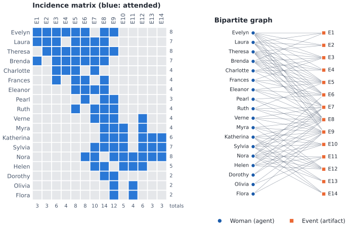
The Davis Southern Women data as an incidence matrix and as a bipartite graph. The margins give each woman’s number of events and each event’s number of women: these degrees drive everything that follows.

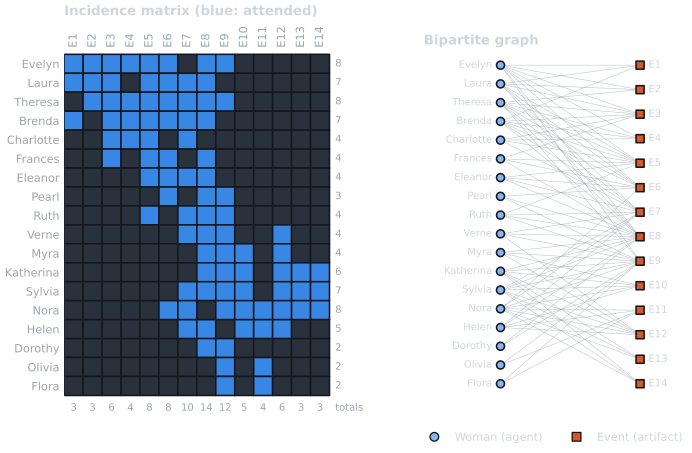
The Davis Southern Women data as an incidence matrix and as a bipartite graph. The margins give each woman’s number of events and each event’s number of women: these degrees drive everything that follows.

Why the raw projection overstates ties

Project the matrix onto the women: the co-occurrence of two women is the number of events both attended, the entries of \(A A^\top\). The simplest projection links every pair with a co-occurrence of at least one. Look at the margins of the matrix first. A few events drew most of the women, and a woman who goes out a lot shares events with nearly everyone. Neither says anything about whom she chose to spend time with.

C = A @ A.T
pairs = [(i, j) for i in range(n_women) for j in range(i + 1, n_women)]
k_obs = np.array([C[i, j] for i, j in pairs])
S = nb.simple_projection(B, women)
largest = int(np.argmax(event_size))
crowded = event_size >= n_women / 2
only_crowded = sum(
    1 for i, j in pairs if C[i, j] > 0 and not (A[i] & A[j] & ~crowded).any()
)
print(f"{len(pairs)} pairs of women; {S.number_of_edges()} co-attend at least once")
print(f"projection density: {nx.density(S):.2f}")
print(
    f"{events[largest]} alone ({event_size[largest]} women) links "
    f"{event_size[largest] * (event_size[largest] - 1) // 2} pairs"
)
print(f"pairs whose shared events all drew at least half the women: {only_crowded}")

153 pairs of women; 139 co-attend at least once
projection density: 0.91
E8 alone (14 women) links 91 pairs
pairs whose shared events all drew at least half the women: 78

Nearly every pair is linked, and many links rest only on crowded events. A backbone keeps the ties that are stronger than expected. To say what is expected, we need two choices: how to weight the projection, and which null model to compare it with.

Projection weights

The projection weight says how much a shared artifact counts. Coscia & Rossi (2019) compare four weightings built from the shared events \(z\) of two women \(u\) and \(v\), where \(d(\cdot)\) is a degree:

• simple: the co-occurrence, \(|\Gamma(u) \cap \Gamma(v)|\);

• hyperbolic: \(\sum_z 1/d(z)\), so a small event counts for more than a crowded one; Newman’s (2001) collaboration weight uses \(1/(d(z) - 1)\) instead;

• ProbS (Zhou et al., 2007): the probability that a two-step random walk from \(u\) (to an event, then to a woman) ends at \(v\), averaged over both directions;

• YCN (Yildirim & Coscia, 2014): the stationary flow of that random walk.

The formulas and calls are in the how-to tutorial; here we look at what they do to the data.

PROJECTIONS = [
    ("simple", "Simple"),
    ("hyper", "Hyperbolic"),
    ("newman", "Newman"),
    ("probs", "ProbS"),
    ("ycn", "YCN"),
]
weights = {
    key: nx.to_numpy_array(
        nb.bipartite_projection(B, women, method=key), nodelist=women, weight="weight"
    )
    for key, _ in PROJECTIONS
}
w_pairs = {key: np.array([W[i, j] for i, j in pairs]) for key, W in weights.items()}
strongest = {key: pairs[int(np.argmax(w))] for key, w in w_pairs.items()}


def pair_name(ij):
    return f"{short[women[ij[0]]]}–{short[women[ij[1]]]}"


watch = sorted({strongest["simple"], strongest["hyper"]})
co = k_obs > 0
print(
    f"{'weighting':<11} {'strongest pair':<18} {'Spearman vs simple':>18}  ranks of",
    end=" ",
)
print(", ".join(pair_name(ij) for ij in watch))
for key, label in PROJECTIONS:
    rank = rankdata(-w_pairs[key], method="min")
    rho = spearmanr(w_pairs[key][co], w_pairs["simple"][co]).statistic
    ranks = ", ".join(str(int(rank[pairs.index(ij)])) for ij in watch)
    print(f"{label:<11} {pair_name(strongest[key]):<18} {rho:>18.2f}  {ranks}")


def draw_projections(mode):
    p = style.palette(mode)
    cmap = style.sequential_cmap(mode).with_extremes(bad=p.hairline)
    fig, axes = plt.subplots(2, 3, figsize=(8.4, 6.2))
    mesh = None
    for ax, (key, label) in zip(axes.flat, PROJECTIONS):
        W = weights[key]
        Z = np.ma.masked_equal(W / W.max(), 0.0)
        mesh = ax.pcolormesh(
            Z, cmap=cmap, vmin=0, vmax=1, edgecolors=p.surface, linewidth=0.4
        )
        ax.set_ylim(n_women, 0)
        ax.set_aspect("equal")
        ax.set_xticks([])
        if ax in axes[:, 0]:
            ax.set_yticks(
                np.arange(n_women) + 0.5, [short[w] for w in women], fontsize=6.5
            )
        else:
            ax.set_yticks([])
        bare(ax)
        ax.set_title(label, pad=14)
        ax.annotate(
            f"strongest: {pair_name(strongest[key])}",
            xy=(0, 1),
            xycoords="axes fraction",
            xytext=(0, 3),
            textcoords="offset points",
            color=p.muted,
            fontsize=7.5,
        )
    key_ax = axes.flat[-1]
    key_ax.set_axis_off()
    cax = key_ax.inset_axes([0.08, 0.62, 0.84, 0.07])
    bar = fig.colorbar(mesh, cax=cax, orientation="horizontal")
    bar.outline.set_visible(False)
    bar.set_label("weight ÷ the panel's largest weight", color=p.ink, fontsize=8)
    key_ax.text(
        0.08,
        0.38,
        "Rows and columns: the women,\nin the order of the incidence matrix.\n"
        "Blank cells: the pair never co-attends\n(and the diagonal).",
        transform=key_ax.transAxes,
        va="top",
        color=p.muted,
        fontsize=8,
    )
    fig.tight_layout()
    return fig


publish(
    "projections",
    draw_projections,
    alt=(
        "Five matrices of pair weights for the women, one per weighting: "
        "simple, hyperbolic, Newman, ProbS and YCN, each scaled to its own "
        "largest weight on a one-hue blue scale. The hyperbolic, Newman "
        "and YCN panels look alike; ProbS emphasizes pairs of women who "
        "attended few events."
    ),
    caption=(
        "The same co-attendance data under five projection weights. Stronger "
        "ties sit at the high end of the color scale; each panel's strongest "
        "pair is named above "
        "it. The table above lists the rank of the simple and hyperbolic "
        "strongest pairs under each weighting."
    ),
)

weighting   strongest pair     Spearman vs simple  ranks of Evelyn–Theresa, Sylvia–Nora
Simple      Evelyn–Theresa                   1.00  1, 2
Hyperbolic  Sylvia–Nora                      0.93  3, 1
Newman      Sylvia–Nora                      0.92  5, 1
ProbS       Katherina–Sylvia                 0.82  6, 3
YCN         Sylvia–Nora                      0.93  3, 1

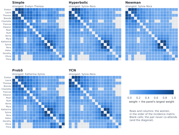
The same co-attendance data under five projection weights. Stronger ties sit at the high end of the color scale; each panel’s strongest pair is named above it. The table above lists the rank of the simple and hyperbolic strongest pairs under each weighting.

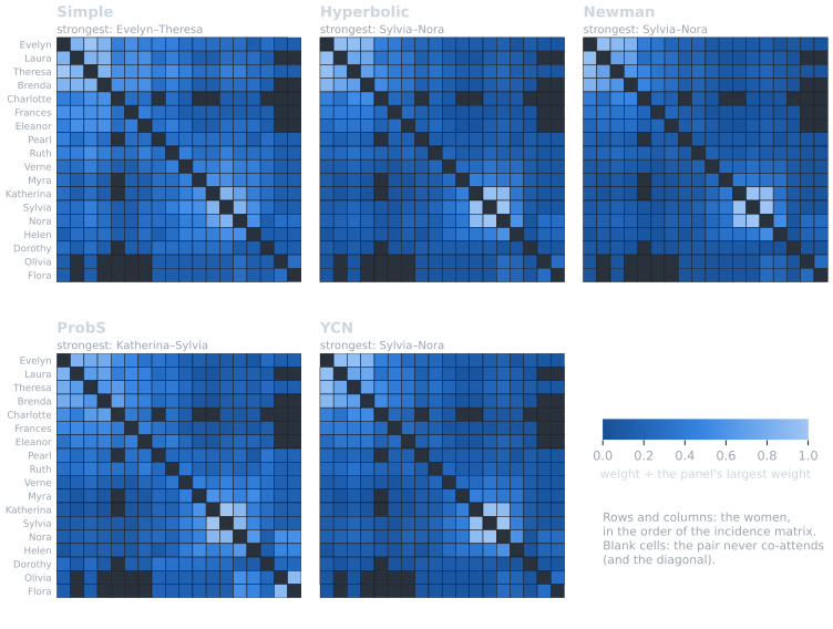
The same co-attendance data under five projection weights. Stronger ties sit at the high end of the color scale; each panel’s strongest pair is named above it. The table above lists the rank of the simple and hyperbolic strongest pairs under each weighting.

The weightings change which ties look strongest: a pair that shares many crowded events leads the simple projection but drops under the hyperbolic weight. Yet none of them says whether a tie is stronger than chance. A weight is a description; to test it, we compare each co-occurrence with its distribution under a null model of the incidence matrix. In nx-backbone the projection weight is only what the returned edges carry (projection=); the test always uses the co-occurrence counts.

Null models

A null model is a family of random incidence matrices that keep some features of the observed one. For each pair of women it gives a distribution of co-occurrences, and the p-value is the chance of a co-occurrence at least as large as the observed one. Neal, Domagalski & Sagan (2021) compare five such models by what they hold fixed:

Model	Women’s degrees	Events’ sizes	How
Fixed fill (FFM)	free	free	only the number of 1s is fixed
Fixed row (FRM)	exact	free	exact (hypergeometric)
Fixed column (FCM)	free	exact	exact (Poisson-binomial)
SDSM	on average	on average	analytic (Poisson-binomial)
FDSM	exact	exact	Monte Carlo

The fixed degree sequence model (FDSM) is the intuitive one: random matrices with exactly the observed row and column sums. It has no formula, so its p-values come from sampling such matrices (here with a curveball Markov chain; Godard & Neal, 2022), which is slow. The stochastic degree sequence model (SDSM; Neal, 2014) keeps both degree sequences only on average: each cell is an independent coin flip whose probability comes from the bipartite configuration model (bicm()), and the co-occurrence is a sum of independent coin flips with a closed-form distribution. Neal et al. found the BiCM probabilities both the fastest and the most accurate of the methods they tried, and the SDSM “a statistically conservative but close approximation” of the FDSM. They recommend the SDSM when the FDSM is impractical. The Backbone 3.0 paper calls the trade of efficiency for power the main consideration between the two, makes the SDSM R’s default, and advises against the three fixed models, which “are known to perform worse”.

Let us see how the five compare on Davis, with the FDSM as the reference.

FDSM_TRIALS = 1000
t0 = time.perf_counter()
H_fdsm = nb.fdsm(B, women, trials=FDSM_TRIALS, seed=42)
seconds = {"FDSM": time.perf_counter() - t0}
scored = {"FDSM": (H_fdsm, "fdsm_pvalue")}
for label, func in [
    ("SDSM", nb.sdsm),
    ("Fixed fill", nb.fixedfill),
    ("Fixed row", nb.fixedrow),
    ("Fixed column", nb.fixedcol),
]:
    t0 = time.perf_counter()
    # The fixed models threshold at alpha themselves; alpha=1 keeps every
    # pair with p < 1, and the pairs left out have p = 1 exactly.
    H = func(B, women) if label == "SDSM" else func(B, women, alpha=1.0)
    seconds[label] = time.perf_counter() - t0
    scored[label] = (H, f"{func.__name__}_pvalue")


def pvalues(H, attr):
    """P-values of every pair, in ``pairs`` order (1 for pairs not returned)."""
    out = np.ones(len(pairs))
    for n, (i, j) in enumerate(pairs):
        if H.has_edge(women[i], women[j]):
            out[n] = H.edges[women[i], women[j]][attr]
    return out


pv = {label: pvalues(H, attr) for label, (H, attr) in scored.items()}
ALPHA = 0.05
kept = {label: set(np.flatnonzero(p < ALPHA)) for label, p in pv.items()}
print(f"{'model':<13} {'kept at 0.05':>12} {'shared with FDSM':>17} {'seconds':>8}")
for label in pv:
    shared = len(kept[label] & kept["FDSM"])
    print(f"{label:<13} {len(kept[label]):>12} {shared:>17} {seconds[label]:>8.3f}")


def draw_nulls(mode):
    p = style.palette(mode)
    others = [label for label in pv if label != "FDSM"]
    lo = min(v[v > 0].min() for v in pv.values()) / 1.8
    fig, axes = plt.subplots(2, 2, figsize=(7.0, 6.6), sharex=True, sharey=True)
    for ax, label in zip(axes.flat, others):
        ax.plot([lo, 1.4], [lo, 1.4], color=p.muted, lw=0.75, zorder=1)
        ax.axhline(ALPHA, color=p.muted, lw=0.6, ls=(0, (2, 2)), zorder=1)
        ax.axvline(ALPHA, color=p.muted, lw=0.6, ls=(0, (2, 2)), zorder=1)
        ax.scatter(
            pv["FDSM"],
            pv[label],
            s=18,
            c=p.kept,
            edgecolors=p.surface,
            linewidths=0.6,
            zorder=2,
        )
        ax.set_xscale("log")
        ax.set_yscale("log")
        ax.set_xlim(lo, 1.4)
        ax.set_ylim(lo, 1.4)
        ax.set_title(label, pad=14)
        shared = len(kept[label] & kept["FDSM"])
        ax.annotate(
            f"keeps {len(kept[label])} pairs, {shared} of them kept by FDSM",
            xy=(0, 1),
            xycoords="axes fraction",
            xytext=(0, 3),
            textcoords="offset points",
            color=p.muted,
            fontsize=7.5,
        )
        ax.text(lo * 1.15, ALPHA * 1.15, "α = 0.05", color=p.muted, fontsize=7.5)
    for ax in axes[1]:
        ax.set_xlabel(f"FDSM p-value ({FDSM_TRIALS} samples)")
    for ax in axes[:, 0]:
        ax.set_ylabel("p-value under the model")
    fig.tight_layout()
    return fig


publish(
    "nulls",
    draw_nulls,
    alt=(
        "Four log-log scatter plots, one per model (SDSM, fixed fill, fixed "
        "row, fixed column), each with one dot per pair of women: FDSM p-value "
        "across, the model's p-value up, a diagonal line of agreement and "
        "dotted lines at 0.05. SDSM dots follow the diagonal from above and "
        "fixed row dots follow it closely; fixed fill and fixed column dots "
        "scatter widely."
    ),
    caption=(
        "Each pair of women's p-value under four null models against its FDSM "
        "p-value. Dots above the diagonal are more conservative than the "
        "FDSM; the bottom-left quadrant holds pairs both models keep at "
        "alpha = 0.05. The counts above each panel match the table printed "
        "above."
    ),
)

model         kept at 0.05  shared with FDSM  seconds
FDSM                     5                 5    0.581
SDSM                     0                 0    0.005
Fixed fill               9                 3    0.004
Fixed row               17                 5    0.001
Fixed column             9                 3    0.001

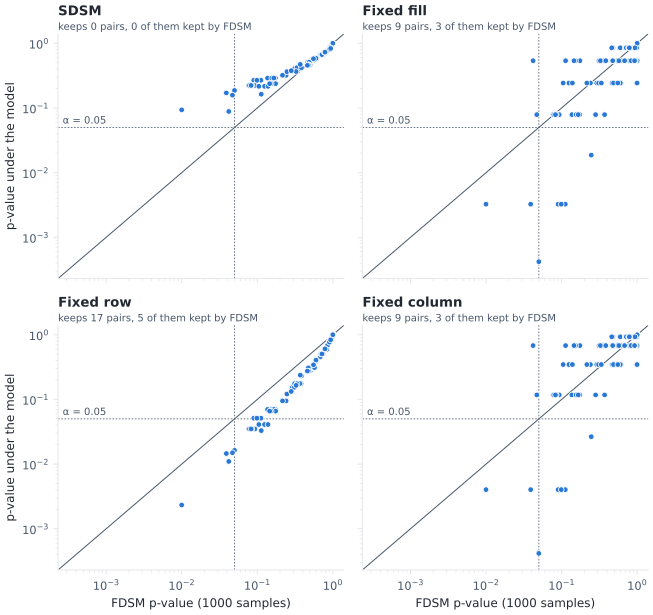
Each pair of women’s p-value under four null models against its FDSM p-value. Dots above the diagonal are more conservative than the FDSM; the bottom-left quadrant holds pairs both models keep at alpha = 0.05. The counts above each panel match the table printed above.

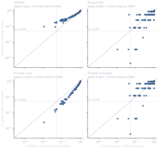
Each pair of women’s p-value under four null models against its FDSM p-value. Dots above the diagonal are more conservative than the FDSM; the bottom-left quadrant holds pairs both models keep at alpha = 0.05. The counts above each panel match the table printed above.

The SDSM tracks the FDSM closely but sits above it: on a matrix this small it keeps no pair at \(\alpha = 0.05\), which is Neal et al.’s “conservative” in action. The fixed fill and fixed column models ignore the women’s degrees, so they reward the women who simply went out more; the fixed row model ignores the events’ sizes and so cannot discount crowded events.

Exact tails and the refined normal approximation

Under the SDSM a co-occurrence follows a Poisson-binomial distribution (a sum of independent coin flips with different probabilities). R backbone evaluates its tail with the refined normal approximation (RNA); nx-backbone computes it exactly by convolution (pvalue_method="auto", the default), and uses the RNA when you ask for it with pvalue_method="rna". On Davis the difference is small but visible (section 7 shows where it is not small):

H_rna = nb.sdsm(B, women, pvalue_method="rna")
p_exact, p_rna = pv["SDSM"], pvalues(H_rna, "sdsm_pvalue")
print(f"smallest p-value: exact {p_exact.min():.4f}, RNA {p_rna.min():.4f}")
print(
    f"largest difference over co-attending pairs: {np.abs(p_exact - p_rna)[co].max():.4f}"
)

smallest p-value: exact 0.0884, RNA 0.0974
largest difference over co-attending pairs: 0.0168

Monte Carlo resolution: the FDSM p-value floor

FDSM p-values are estimated from trials sampled matrices as \((\text{count} + 1) / (\text{trials} + 1)\), so none can fall below the floor \(1/(\text{trials} + 1)\). On Davis the floor does not bind. It does once we correct for multiple testing. With \(m\) pairs, Bonferroni and Holm need a p-value below \(\alpha / m\), so with fewer than about \(m / \alpha\) trials no pair can pass, whatever the data.

To see it, plant a group of agents who share a block of artifacts in an otherwise random incidence matrix, and score it with more and more trials. (A warning for this case is planned in issue #76; for now the check is yours to make.)

rng = np.random.default_rng(2)
R = (rng.random((48, 80)) < 0.08).astype(np.int8)
R[:8, :20] = rng.random((8, 20)) < 0.95
m = R.shape[0] * (R.shape[0] - 1) // 2
H_sdsm_R = nb.sdsm(R)
sdsm_min = min(d["sdsm_pvalue"] for *_, d in H_sdsm_R.edges(data=True))
needed = int(np.ceil(m / ALPHA - 1))
print(
    f"{R.shape[0]} agents x {R.shape[1]} artifacts, m = {m} pairs, alpha/m = {ALPHA / m:.1e}"
)
print(
    f"smallest SDSM p-value: {sdsm_min:.1e}; FDSM needs >= {needed} trials to go below alpha/m"
)
print(
    f"{'trials':>7} {'floor':>9} {'smallest p':>11} {'pairs at floor':>15} {'seconds':>8}"
)
floor_rows = []
for trials in (10, 40, 160, 640):
    t0 = time.perf_counter()
    H_fdsm_R = nb.fdsm(R, trials=trials, seed=7)
    elapsed = time.perf_counter() - t0
    p_R = np.array([d["fdsm_pvalue"] for *_, d in H_fdsm_R.edges(data=True)])
    floor = 1 / (trials + 1)
    at_floor = int(np.isclose(p_R, floor).sum())
    floor_rows.append((trials, p_R.min(), at_floor))
    print(
        f"{trials:>7} {floor:>9.1e} {p_R.min():>11.1e} {at_floor:>15} {elapsed:>8.2f}"
    )

print(
    f"\nkept at alpha = {ALPHA} after correcting for {m} tests ({floor_rows[-1][0]} trials):"
)
for mtc in ("holm", "bh"):
    n_fdsm = nb.threshold_filter(
        H_fdsm_R, "fdsm_pvalue", ALPHA, mtc=mtc
    ).number_of_edges()
    n_sdsm = nb.threshold_filter(
        H_sdsm_R, "sdsm_pvalue", ALPHA, mtc=mtc
    ).number_of_edges()
    print(f"  {mtc:<5} FDSM {n_fdsm:>3}   SDSM {n_sdsm:>3}")


def draw_floor(mode):
    p = style.palette(mode)
    fdsm_color, sdsm_color = style.categorical(2, mode)
    fig, ax = plt.subplots(figsize=(6.6, 4.0))
    x = np.geomspace(10, needed * 3, 200)
    ax.plot(x, 1 / (x + 1), color=p.muted, lw=1.0, label="floor 1/(trials + 1)")
    ax.axhline(
        ALPHA / m,
        color=p.ink,
        lw=0.75,
        ls=(0, (4, 2)),
        label="Bonferroni and Holm need p < α/m",
    )
    ax.axhline(
        sdsm_min, color=sdsm_color, lw=1.5, label="smallest SDSM p-value (no floor)"
    )
    t_runs = [r[0] for r in floor_rows]
    ax.plot(
        t_runs,
        [r[1] for r in floor_rows],
        marker="o",
        color=fdsm_color,
        markeredgecolor=p.surface,
        label="smallest FDSM p-value",
    )
    for t, pmin, n in floor_rows:
        ax.annotate(
            f"{n} pairs\nat floor",
            (t, pmin),
            xytext=(6, 4),
            textcoords="offset points",
            fontsize=7,
            color=p.muted,
        )
    ax.plot([needed], [ALPHA / m], marker="o", color=p.ink, markersize=4, linestyle="")
    ax.annotate(
        f"≈ {needed:,} trials",
        (needed, ALPHA / m),
        xytext=(-4, 6),
        textcoords="offset points",
        ha="right",
        fontsize=7.5,
        color=p.ink,
    )
    ax.text(12, sdsm_min * 1.25, "SDSM", fontsize=7.5, color=p.ink)
    ax.set_xscale("log")
    ax.set_yscale("log")
    ax.set_ylim(top=0.6)
    ax.set_xlabel("FDSM trials")
    ax.set_ylabel("p-value")
    ax.grid(True, which="major")
    ax.set_title("No FDSM p-value can go below 1/(trials + 1)")
    ax.legend(loc="upper center", bbox_to_anchor=(0.5, -0.18), ncols=2)
    return fig


publish(
    "floor",
    draw_floor,
    alt=(
        f"Log-log line chart of p-value against FDSM trials for a {R.shape[0]} "
        f"by {R.shape[1]} planted-block matrix. The smallest FDSM p-value sits "
        "exactly on the falling floor line 1/(trials + 1) at every trial "
        "count. A horizontal dashed line marks alpha/m, which the floor only "
        f"reaches at about {needed:,} trials; a horizontal orange line marks "
        "the smallest SDSM p-value."
    ),
    caption=(
        "The FDSM p-value floor on a planted-block matrix. Every run's "
        "smallest p-value is the floor itself, shared by the pairs labeled. "
        "With fewer trials than marked on the alpha/m line, Bonferroni and "
        "Holm cannot keep any pair."
    ),
)

48 agents x 80 artifacts, m = 1128 pairs, alpha/m = 4.4e-05
smallest SDSM p-value: 1.6e-05; FDSM needs >= 22559 trials to go below alpha/m
 trials     floor  smallest p  pairs at floor  seconds
     10   9.1e-02     9.1e-02              54     0.02
     40   2.4e-02     2.4e-02              30     0.07
    160   6.2e-03     6.2e-03              28     0.27
    640   1.6e-03     1.6e-03              27     1.05

kept at alpha = 0.05 after correcting for 1128 tests (640 trials):
  holm  FDSM   0   SDSM   4
  bh    FDSM   0   SDSM  10

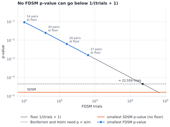
The FDSM p-value floor on a planted-block matrix. Every run’s smallest p-value is the floor itself, shared by the pairs labeled. With fewer trials than marked on the alpha/m line, Bonferroni and Holm cannot keep any pair.

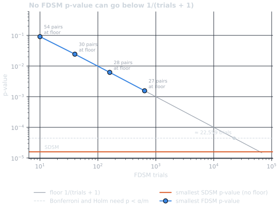
The FDSM p-value floor on a planted-block matrix. Every run’s smallest p-value is the floor itself, shared by the pairs labeled. With fewer trials than marked on the alpha/m line, Bonferroni and Holm cannot keep any pair.

The FDSM’s smallest p-value is never a measurement here: it is the floor, shared by a whole group of pairs at once. A family-wise correction then keeps nothing. The BH correction compares the \(k\)-th smallest p-value with \(k\alpha/m\), so it keeps the pairs tied at the floor all together or not at all, depending on how many are tied, not on how strong each tie is. Either use enough trials (about \(m/\alpha\)), or use the SDSM, whose analytic p-values have no floor.

Signed backbones of the projection

So far each test was one-tailed: it asks whether two women co-attend more than expected. A two-tailed test also finds pairs who co-attend significantly less than expected, women who seem to avoid each other’s events. With signed=True the stored p-value is two-sided and each edge gets a "sign": +1 for a significantly strong tie, -1 for a significantly weak one. A pair that never co-attends can still be significantly weak, so a signed backbone can contain ties the projection does not.

H_signed = nb.fdsm(B, women, trials=FDSM_TRIALS, seed=42, signed=True)
signed_bb = nb.threshold_filter(H_signed, "fdsm_pvalue", ALPHA)
sign = np.zeros((n_women, n_women), dtype=int)
idx = {w: i for i, w in enumerate(women)}
for u, v, d in signed_bb.edges(data=True):
    sign[idx[u], idx[v]] = sign[idx[v], idx[u]] = d["sign"]
n_pos = int((sign > 0).sum() // 2)
n_neg = int((sign < 0).sum() // 2)
print(
    f"signed FDSM backbone at alpha = {ALPHA}: {n_pos} positive, {n_neg} negative ties"
)
print(f"{'pair':<22} {'co-attend':>9} {'sign':>5} {'p':>7}")
for u, v, d in sorted(
    signed_bb.edges(data=True), key=lambda e: (-e[2]["sign"], e[2]["fdsm_pvalue"])
):
    print(
        f"{short[u] + '–' + short[v]:<22} {C[idx[u], idx[v]]:>9} {d['sign']:>+5} {d['fdsm_pvalue']:>7.3f}"
    )
pos_layout = style.layout(S, "davis_women", weight="weight")


def draw_signed(mode):
    p = style.palette(mode)
    fig, (ax, gx) = plt.subplots(
        1, 2, figsize=(8.4, 4.6), gridspec_kw={"width_ratios": [1, 1.05]}
    )
    ax.pcolormesh(
        sign,
        cmap=ListedColormap([p.negative, p.hairline, p.positive]),
        vmin=-1.5,
        vmax=1.5,
        edgecolors=p.surface,
        linewidth=0.8,
    )
    for i in range(n_women):
        for j in range(n_women):
            if sign[i, j]:
                ax.text(
                    j + 0.5,
                    i + 0.52,
                    "+" if sign[i, j] > 0 else "−",
                    ha="center",
                    va="center",
                    color=p.surface,
                    fontsize=8,
                    fontweight="bold",
                )
    ax.set_ylim(n_women, 0)
    ax.set_aspect("equal")
    ax.set_xticks(
        np.arange(n_women) + 0.5, [short[w] for w in women], rotation=90, fontsize=7
    )
    ax.set_yticks(np.arange(n_women) + 0.5, [short[w] for w in women], fontsize=7)
    bare(ax)
    ax.set_title("Sign of each significant pair")

    counts = style.draw_backbone(
        gx, H_signed, signed_bb, pos_layout, mode=mode, sign="sign"
    )
    for w, (x, y) in pos_layout.items():
        gx.annotate(
            short[w],
            (x, y),
            xytext=(0, 5),
            textcoords="offset points",
            ha="center",
            fontsize=6.5,
        )
    gx.set_title("Signed backbone over all tested pairs", pad=16)
    gx.annotate(
        counts.short,
        xy=(0, 1),
        xycoords="axes fraction",
        xytext=(0, 6),
        textcoords="offset points",
        va="bottom",
        color=p.muted,
        fontsize=7.5,
    )
    fig.tight_layout()
    return fig


publish(
    "signed",
    draw_signed,
    alt=(
        f"Left: an {n_women} by {n_women} matrix of the women with {n_pos} "
        f"pairs marked + on blue (significantly strong) and {n_neg} pairs "
        "marked − on red (significantly weak). Right: the same ties drawn as "
        "a network over faint lines for every tested pair, positive ties solid "
        "blue and negative ties dashed red."
    ),
    caption=(
        "A signed FDSM backbone of the Davis projection at alpha = 0.05 "
        "(two-sided). Positive ties are blue with a + (solid lines); negative "
        "ties are red with a − (dashed lines)."
    ),
)
_ = style.save_variants(
    draw_signed, IMAGES / "bipartite_thumb", fmt="png", modes=("light",)
)

signed FDSM backbone at alpha = 0.05: 1 positive, 8 negative ties
pair                   co-attend  sign       p
Katherina–Sylvia               6    +1   0.020
Evelyn–Nora                    2    -1   0.012
Laura–Nora                     2    -1   0.020
Brenda–Katherina               1    -1   0.026
Charlotte–Katherina            0    -1   0.030
Katherina–Laura                1    -1   0.038
Evelyn–Sylvia                  2    -1   0.040
Brenda–Nora                    2    -1   0.042
Evelyn–Helen                   1    -1   0.046

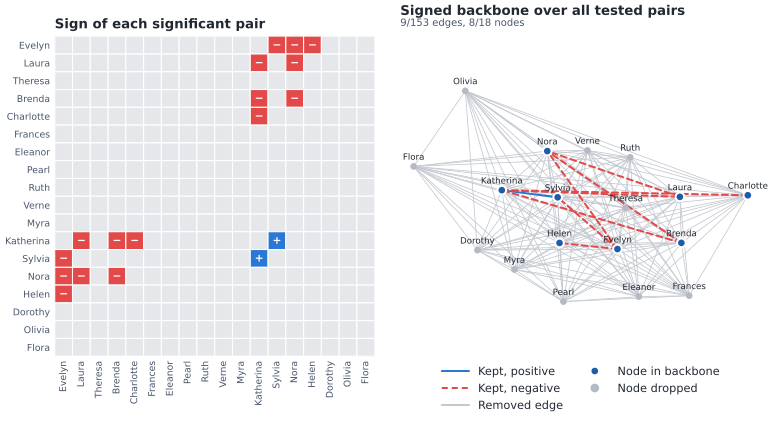
A signed FDSM backbone of the Davis projection at alpha = 0.05 (two-sided). Positive ties are blue with a + (solid lines); negative ties are red with a − (dashed lines).

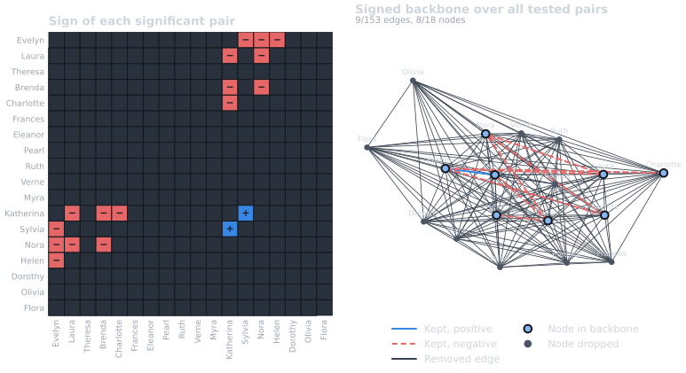
A signed FDSM backbone of the Davis projection at alpha = 0.05 (two-sided). Positive ties are blue with a + (solid lines); negative ties are red with a − (dashed lines).

The negative ties are as informative as the positive ones: they mark women who move in different circles. A one-tailed backbone would show only the strong ties within each circle. Signed backbones are available for sdsm(), fdsm() and the three fixed models, and through backbone_from_projection() with signed=True.

SDSM-EC: when some cells cannot vary

Every null model so far lets any woman attend any event. Real data often has structural zeros and ones: a person who joined an organization late could not have attended its early meetings, and a host had to attend her own party. Treating such cells as free makes the null model wrong in a predictable way. The SDSM with edge constraints (SDSM-EC; Neal & Neal, 2023) fixes them: prohibited cells have null probability 0 and required cells have probability 1, and the BiCM is fitted on the remaining cells.

Suppose, as a thought experiment, that the women who first appear at the largest event or later had only then arrived in town, so they could not have attended anything earlier, and that the first two women on the list who attended the largest event hosted it, so they had to be there.

first_event = {w: min(events.index(e) for e in B[w]) for w in women}
host_event = events[largest]
late = [w for w in women if first_event[w] >= largest]
hosts = [w for w in women if B.has_edge(w, host_event)][:2]
prohibited = [(w, events[k]) for w in late for k in range(largest)]
required = [(w, host_event) for w in hosts]
print("arrived late:", ", ".join(short[w] for w in late))
print(f"hosts of {host_event}:", ", ".join(short[w] for w in hosts))
print(f"{len(prohibited)} prohibited and {len(required)} required cells")

H_ec = nb.sdsm(B, women, prohibited=prohibited, required=required)
p_ec = pvalues(H_ec, "sdsm_pvalue")
involves_late = np.array([women[i] in late or women[j] in late for i, j in pairs])
change = p_ec - p_exact
print(f"{'pair':<20} {'SDSM p':>7} {'SDSM-EC p':>10}")
for n in np.argsort(-np.abs(change))[:6]:
    print(f"{pair_name(pairs[n]):<20} {p_exact[n]:>7.3f} {p_ec[n]:>10.3f}")
print(f"smallest p-value: SDSM {p_exact.min():.3f}, SDSM-EC {p_ec.min():.3f}", end=" ")
print(f"({pair_name(pairs[int(np.argmin(p_ec))])})")


def draw_constraints(mode):
    p = style.palette(mode)
    late_color, other_color = style.categorical(2, mode)
    fig, (ax, sx) = plt.subplots(
        1, 2, figsize=(8.4, 4.4), gridspec_kw={"width_ratios": [1, 1.05]}
    )
    ax.pcolormesh(
        A,
        cmap=ListedColormap([p.hairline, p.kept]),
        vmin=0,
        vmax=1,
        edgecolors=p.surface,
        linewidth=1.0,
    )
    px = [events.index(e) + 0.5 for _, e in prohibited]
    py = [idx[w] + 0.5 for w, _ in prohibited]
    ax.scatter(
        px,
        py,
        marker="x",
        s=16,
        c=p.ink,
        linewidths=1.0,
        label="prohibited (could not attend)",
    )
    rx = [events.index(e) + 0.5 for _, e in required]
    ry = [idx[w] + 0.5 for w, _ in required]
    ax.scatter(
        rx,
        ry,
        marker="o",
        s=26,
        facecolors="none",
        edgecolors=p.surface,
        linewidths=1.6,
        label="required (had to attend)",
    )
    ax.set_ylim(n_women, 0)
    ax.set_aspect("equal")
    ax.set_xticks(np.arange(n_events) + 0.5, events, rotation=90, fontsize=7)
    ax.set_yticks(np.arange(n_women) + 0.5, [short[w] for w in women], fontsize=7)
    ax.xaxis.tick_top()
    bare(ax)
    ax.set_title("Constrained cells", pad=24)
    handles = [
        Line2D(
            [],
            [],
            marker="s",
            linestyle="",
            markerfacecolor=p.kept,
            markeredgecolor=p.kept,
            label="attended",
        ),
        Line2D(
            [],
            [],
            marker="x",
            linestyle="",
            color=p.ink,
            label="prohibited (could not attend)",
        ),
        (
            Line2D(
                [],
                [],
                marker="s",
                linestyle="",
                markersize=9,
                markerfacecolor=p.kept,
                markeredgecolor=p.kept,
            ),
            Line2D(
                [],
                [],
                marker="o",
                linestyle="",
                markersize=5,
                markerfacecolor="none",
                markeredgecolor=p.surface,
                markeredgewidth=1.4,
            ),
        ),
    ]
    labels = ["attended", "prohibited (could not attend)", "required (had to attend)"]
    ax.legend(
        handles=handles,
        labels=labels,
        loc="upper center",
        bbox_to_anchor=(0.5, -0.02),
        ncols=1,
    )

    sx.plot([0, 1.02], [0, 1.02], color=p.muted, lw=0.75, zorder=1)
    for mask, color, marker, label in [
        (~involves_late & co, other_color, "^", "other pairs"),
        (involves_late & co, late_color, "o", "pairs with a late arrival"),
    ]:
        sx.scatter(
            p_exact[mask],
            p_ec[mask],
            s=22,
            c=color,
            marker=marker,
            edgecolors=p.surface,
            linewidths=0.6,
            label=label,
            zorder=2,
        )
    sx.set_xlim(0, 1.02)
    sx.set_ylim(0, 1.02)
    sx.set_aspect("equal")
    sx.set_xlabel("SDSM p-value")
    sx.set_ylabel("SDSM-EC p-value")
    sx.set_title("Co-attending pairs, before and after")
    sx.legend(loc="upper center", bbox_to_anchor=(0.5, -0.16), ncols=2)
    fig.tight_layout()
    return fig


publish(
    "constraints",
    draw_constraints,
    alt=(
        "Left: the incidence matrix with crosses on the cells of the women who "
        "arrived late, for every event before the largest one, and white rings "
        "on the two hosts' cells for that event. Right: a scatter of each "
        "co-attending pair's SDSM p-value across and SDSM-EC p-value up, "
        "blue circles for pairs with a late arrival and orange triangles for "
        "the others, around a diagonal line."
    ),
    caption=(
        "SDSM-EC on a thought experiment. Left: prohibited cells (crosses) and "
        "required cells (rings). Right: how each co-attending pair's p-value "
        "moves once those cells are fixed; dots on the diagonal line do not "
        "move. The pairs that move most are listed in the table above."
    ),
)

arrived late: Myra, Katherina, Dorothy, Olivia, Flora
hosts of E8: Evelyn, Laura
35 prohibited and 2 required cells
pair                  SDSM p  SDSM-EC p
Myra–Katherina         0.158      0.521
Katherina–Helen        0.577      0.261
Verne–Katherina        0.420      0.142
Katherina–Dorothy      0.366      0.638
Pearl–Katherina        0.589      0.327
Myra–Dorothy           0.238      0.498
smallest p-value: SDSM 0.088, SDSM-EC 0.005 (Katherina–Sylvia)

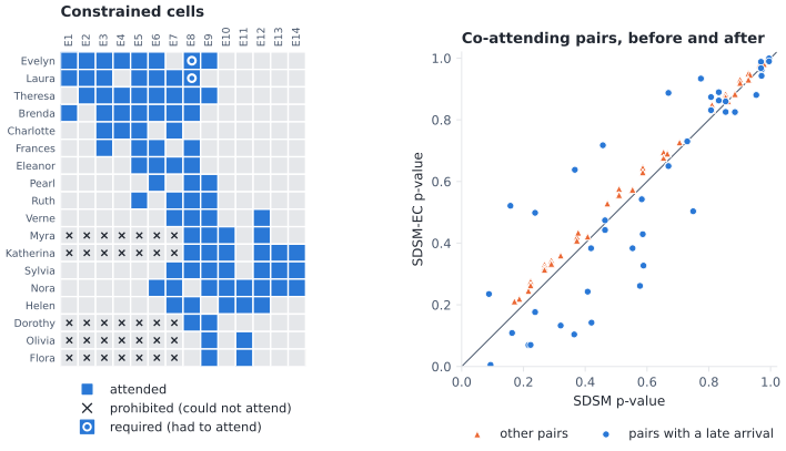
SDSM-EC on a thought experiment. Left: prohibited cells (crosses) and required cells (rings). Right: how each co-attending pair’s p-value moves once those cells are fixed; dots on the diagonal line do not move. The pairs that move most are listed in the table above.

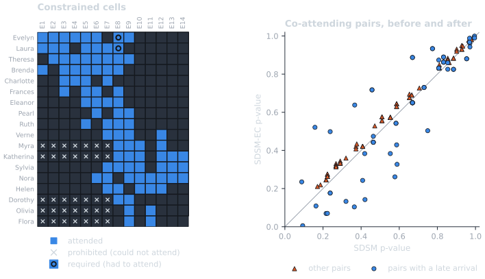
SDSM-EC on a thought experiment. Left: prohibited cells (crosses) and required cells (rings). Right: how each co-attending pair’s p-value moves once those cells are fixed; dots on the diagonal line do not move. The pairs that move most are listed in the table above.

Fixing cells moves each pair’s expected co-occurrence, and the p-values move in both directions. Once the late arrivals could not have gone to the early events, their attendance is concentrated on fewer events, so two late arrivals meeting there is less surprising, while a late arrival meeting a woman who was free to attend everything can become more surprising. The hosts’ attendance stops counting as evidence of anything. The constraints change the question, not just the answer, so they must come from knowledge of how the data was produced, never from the data itself.

Contradictory constraints

A constraint must agree with the data: a prohibited cell cannot be an observed attendance, and a required cell must be one. A constraint that contradicts the data is ignored, with one RuntimeWarning that counts and lists the ignored pairs, and the other constraints are kept. A cell that is both required and prohibited is an error in the constraints themselves and raises NetworkXError.

attended, missed = women[0], women[-1]
first_of = events[first_event[attended]]
assert B.has_edge(attended, first_of) and not B.has_edge(missed, first_of)
with warnings.catch_warnings(record=True) as caught:
    warnings.simplefilter("always")
    H_bad = nb.sdsm(
        B, women, prohibited=[(attended, first_of)], required=[(missed, first_of)]
    )
for w in caught:
    print(f"{w.category.__name__}: {w.message}")
print(
    "same as the unconstrained SDSM:",
    np.allclose(pvalues(H_bad, "sdsm_pvalue"), p_exact),
)
try:
    nb.sdsm(
        B, women, prohibited=[(attended, first_of)], required=[(attended, first_of)]
    )
except nx.NetworkXError as err:
    print(f"NetworkXError: {err}")

RuntimeWarning: sdsm: ignoring SDSM-EC constraints that contradict the data: 1 required pair(s) that are not edges of B [('Flora Price', 'E1')]; 1 prohibited pair(s) that are edges of B [('Evelyn Jefferson', 'E1')].
same as the unconstrained SDSM: True
NetworkXError: sdsm: 1 pair(s) are both required and prohibited: ('Evelyn Jefferson', 'E1').

Matching R

The R package backbone (Neal, 2022) is the reference implementation of these models, and nx-backbone’s test suite checks its p-values and backbones against fixtures computed with R backbone on the same Davis data (tests/test_reference_implementations.py; see Contributing to regenerate them). Here we read those fixtures directly. Where an exact p-value is cheap, nx-backbone computes it exactly, so it can differ from R’s approximation by design; with pvalue_method="rna" the SDSM agrees with R to the precision of the BiCM fit.

fixture = json.loads(
    (DOCS.parent / "tests" / "fixtures" / "r_backbone.json").read_text("utf-8")
)
davis_r = fixture["davis"]
assert davis_r["agents"] == women
r_pairs = [tuple(ij) for ij in davis_r["pairs"]]
assert r_pairs == pairs
r_k = np.array(davis_r["cooccurrence"])
print(f"R backbone {fixture['meta']['backbone']} (R {fixture['meta']['R']})")
comparisons = [
    ("SDSM, RNA tail", p_rna, np.array(davis_r["sdsm"]["upper"], dtype=float), r_k > 0),
    (
        "SDSM, exact tail (default)",
        p_exact,
        np.array(davis_r["sdsm"]["upper"], dtype=float),
        r_k > 0,
    ),
    (
        "Fixed fill",
        pv["Fixed fill"],
        np.array(davis_r["fixedfill"]["upper"], dtype=float),
        r_k >= 0,
    ),
]
for label, ours, theirs, mask in comparisons:
    print(f"{label:<28} largest |difference| {np.abs(ours - theirs)[mask].max():.1e}")


def draw_r(mode):
    p = style.palette(mode)
    fig, axes = plt.subplots(1, 3, figsize=(8.4, 3.3), sharex=True, sharey=True)
    for ax, (label, ours, theirs, mask) in zip(axes, comparisons):
        ax.plot([0, 1], [0, 1], color=p.muted, lw=0.75, zorder=1)
        ax.scatter(
            theirs[mask],
            ours[mask],
            s=16,
            c=p.kept,
            edgecolors=p.surface,
            linewidths=0.6,
            zorder=2,
        )
        ax.set_xlim(0, 1.02)
        ax.set_ylim(0, 1.02)
        ax.set_aspect("equal")
        ax.set_title(label, pad=14, fontsize=9)
        ax.annotate(
            f"largest gap {np.abs(ours - theirs)[mask].max():.1e}",
            xy=(0, 1),
            xycoords="axes fraction",
            xytext=(0, 3),
            textcoords="offset points",
            color=p.muted,
            fontsize=7.5,
        )
        ax.set_xlabel("R backbone p-value")
    axes[0].set_ylabel("nx-backbone p-value")
    fig.tight_layout()
    return fig


publish(
    "r_match",
    draw_r,
    alt=(
        "Three scatter plots of nx-backbone p-values up against R "
        "backbone p-values across, one dot per pair of Davis women, with a "
        "diagonal line. In the SDSM RNA panel and the fixed fill panel every "
        "dot lies on the diagonal; in the exact SDSM panel the dots sit "
        "slightly off it."
    ),
    caption=(
        "nx-backbone against R backbone on Davis. The SDSM panels show "
        "the pairs that co-attend; R does not test the others by default."
    ),
)

R backbone 3.0.4 (R 4.3.3)
SDSM, RNA tail               largest |difference| 2.4e-09
SDSM, exact tail (default)   largest |difference| 1.7e-02
Fixed fill                   largest |difference| 2.4e-14

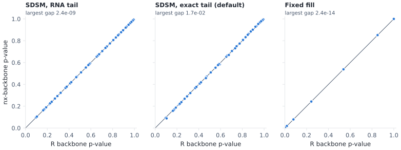
nx-backbone against R backbone on Davis. The SDSM panels show the pairs that co-attend; R does not test the others by default.

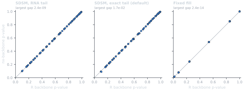
nx-backbone against R backbone on Davis. The SDSM panels show the pairs that co-attend; R does not test the others by default.

Which pairs are tested: missing_as_zero

One convention changes results without changing any p-value: which pairs count as tests. R backbone_from_projection by default (missing_as_zero = FALSE) tests only pairs that co-occur at least once. nx-backbone by default tests every pair, including those that never co-occur. Without a correction and without signed=True the two give the same backbone, because a pair that never co-occurs has an upper-tail p-value of 1. With a multiple-testing correction, fewer tests make the correction less strict, and with signed=True a pair that never co-occurs can be significantly weak. Pass missing_as_zero=False to reproduce R’s default.

def backbone_set(H):
    return {(frozenset(e), H.edges[e].get("sign", 1)) for e in H.edges}


def r_set(entries):
    return {(frozenset((women[i], women[j])), s) for i, j, s in entries}


maz = davis_r["missing_as_zero"]
alpha_maz = maz["alphas"][0]
print(
    f"never co-attend: {int((k_obs == 0).sum())} of {len(pairs)} pairs; alpha = {alpha_maz}"
)
print(f"{'model':<10} {'mtc':<11} {'all pairs':>9} {'co-occurring':>13} {'= R':>4}")
for model in ("fixedfill", "fixedrow"):
    for mtc in ("none", "bonferroni", "holm", "BH"):
        counts, same = [], True
        for flag in (True, False):
            H = nb.backbone_from_projection(
                B, women, method=model, alpha=alpha_maz, mtc=mtc, missing_as_zero=flag
            )
            counts.append(H.number_of_edges())
            same &= backbone_set(H) == r_set(
                maz[model][str(flag).lower()][str(alpha_maz)][mtc]
            )
        print(
            f"{model:<10} {mtc:<11} {counts[0]:>9} {counts[1]:>13} {'yes' if same else 'NO':>4}"
        )

never co-attend: 14 of 153 pairs; alpha = 0.06
model      mtc         all pairs  co-occurring  = R
fixedfill  none                9             9  yes
fixedfill  bonferroni          0             1  yes
fixedfill  holm                0             1  yes
fixedfill  BH                  0             8  yes
fixedrow   none               22            22  yes
fixedrow   bonferroni          0             0  yes
fixedrow   holm                0             0  yes
fixedrow   BH                  0             0  yes

Each row compares both settings with the matching R run, and they agree. Choose missing_as_zero=False when you want R’s numbers, and keep the default when a pair that never co-occurs is as much a test as any other.

Scale: sparse incidence matrices

Every function on this page also accepts an agents x artifacts incidence matrix: a NumPy array, a SciPy sparse array or matrix, or a pandas DataFrame. The matrix stays sparse, co-occurrences come from sparse products, and agent pairs are scored in blocks of rows. backbone_from_projection() turns only the significant pairs into edges, so memory stays bounded; sdsm() and fdsm() return every pair as an edge, which is only practical for a few thousand agents.

The run below plants a group of agents who share a block of artifacts in sparse random matrices and asks the SDSM for a backbone with the BH correction (Benjamini & Hochberg, 1995), which millions of tests make necessary. A matrix this sparse needs care with the tail: each pair’s expected co-occurrence is tiny, far from the normal shape the RNA assumes. Compare the default (pvalue_method="auto", exact here) with the RNA that R backbone uses:

rng = np.random.default_rng(0)
group = 30
planted = group * (group - 1) // 2
print(
    f"{'agents':>6} {'artifacts':>9} {'pairs':>10} {'nonzeros':>9} {'tail':>6} "
    f"{'kept':>6} {'planted':>8} {'other':>6} {'seconds':>8}"
)
scale_rows = []
for n_agents in (1000, 2000):
    n_artifacts = n_agents // 4
    M = sp.random_array((n_agents, n_artifacts), density=0.01, format="lil", rng=rng)
    M[:group, :40] = (rng.random((group, 40)) < 0.5).astype(float)
    M = M.tocsr()
    M.data[:] = 1.0
    M.eliminate_zeros()
    n_pairs = n_agents * (n_agents - 1) // 2
    for tail in ("auto", "rna"):
        t0 = time.perf_counter()
        bh = nb.backbone_from_projection(
            M, method="sdsm", alpha=ALPHA, mtc="bh", pvalue_method=tail
        )
        elapsed = time.perf_counter() - t0
        found = sum(1 for u, v in bh.edges() if u < group and v < group)
        other = bh.number_of_edges() - found
        scale_rows.append((n_agents, tail, found, other))
        print(
            f"{n_agents:>6} {n_artifacts:>9} {n_pairs:>10,} {M.nnz:>9,} {tail:>6} "
            f"{bh.number_of_edges():>6,} {found:>4} of {planted} {other:>6,} {elapsed:>8.2f}"
        )

agents artifacts      pairs  nonzeros   tail   kept  planted  other  seconds
  1000       250    499,500     3,084   auto     83   83 of 435      0     0.10
  1000       250    499,500     3,084    rna    395  234 of 435    161     0.08
  2000       500  1,999,000    10,603   auto    304  304 of 435      0     0.23
  2000       500  1,999,000    10,603    rna  1,826  391 of 435  1,435     0.26

“Planted” counts the pairs inside the planted group that the backbone keeps; “other” counts every other pair it keeps, all of them noise here. The default, exact tail keeps (almost) only planted pairs. The RNA reports p-values far smaller than the true ones for pairs with a tiny expected co-occurrence, so noise pairs pass even a corrected test. Use pvalue_method="rna" only to reproduce R’s numbers.

The exact tail stays cheap because a convolution only needs to run up to the largest co-occurrence two agents can have (the smaller of their degrees), once per pair of distinct agent degrees. Until issue #108 was fixed, "auto" switched to the RNA above 200 artifacts, as in this table’s RNA rows. Now it does so only for pairs whose exact tail would be too costly, starting with the largest expected co-occurrences (where the RNA is accurate), and warns when it does.

Where next

• Bipartite Projection Backbones: the how-to reference for every call on this page (projections, SDSM, FDSM, the fixed models, signed backbones, SDSM-EC, incidence-matrix input).

• Bipartite Methods: the API reference, including backbone_from_projection(), sdsm(), fdsm(), bicm() and fastball().

• Choosing a Method and Workflow: where projection backbones fit among the other methods, and the score-then-filter workflow.

• Hypergraph Backbones: hypergraphs project onto their nodes in the same way and use the same null models.

• Validating a Backbone: checking that a backbone is not an artifact of the choices made here.

• describe_backbone(): methods text and citations for the backbone you report.

References

• Benjamini, Y., & Hochberg, Y. (1995). Controlling the false discovery rate: a practical and powerful approach to multiple testing. Journal of the Royal Statistical Society: Series B, 57(1), 289-300.

• Coscia, M., & Rossi, L. (2019). The impact of projection and backboning on network topologies. Proceedings of the IEEE/ACM International Conference on Advances in Social Networks Analysis and Mining (ASONAM). https://doi.org/10.1145/3341161.3342862

• Godard, K., & Neal, Z. P. (2022). fastball: A fast algorithm to sample bipartite graphs with fixed degree sequences. Journal of Complex Networks, 10(6), cnac049. https://doi.org/10.1093/comnet/cnac049

• Neal, Z. P. (2014). The backbone of bipartite projections: Inferring relationships from co-authorship, co-sponsorship, co-attendance and other co-behaviors. Social Networks, 39, 84-97. https://doi.org/10.1016/j.socnet.2014.06.001

• Neal, Z. P. (2022). backbone: An R package to extract network backbones. PLoS ONE, 17(5), e0269137. https://doi.org/10.1371/journal.pone.0269137

• Neal, Z. P. (2026). Backbone 3.0: An R package for extracting network backbones. PLoS ONE, 21(5), e0349258. https://doi.org/10.1371/journal.pone.0349258

• Neal, Z. P., & Neal, J. W. (2023). Stochastic Degree Sequence Model with Edge Constraints (SDSM-EC) for Backbone Extraction. Complex Networks XII, 127-136. https://doi.org/10.1007/978-3-031-53468-3_11

• Neal, Z. P., Domagalski, R., & Sagan, B. (2021). Comparing alternatives to the fixed degree sequence model for extracting the backbone of bipartite projections. Scientific Reports, 11, 23929. https://doi.org/10.1038/s41598-021-03238-3

• Newman, M. E. J. (2001). Scientific collaboration networks. II. Shortest paths, weighted networks, and centrality. Physical Review E, 64, 016132.

• Yildirim, M. A., & Coscia, M. (2014). Using random walks to generate associations between objects. PLoS ONE, 9(8), e104813. https://doi.org/10.1371/journal.pone.0104813

• Zhou, T., Ren, J., Medo, M., & Zhang, Y.-C. (2007). Bipartite network projection and personal recommendation. Physical Review E, 76, 046115. https://doi.org/10.1103/PhysRevE.76.046115