Proximity Methods

Examples in this module use nx.les_miserables_graph(). Methods return scored full graphs; typical extraction uses fraction_filter() on similarity attributes. Complexity classes are provided in each function docstring.

Proximity-based edge scoring methods.

These methods score each existing edge by the topological proximity (similarity) of its endpoints. They are useful for identifying structurally embedded edges (high proximity) versus bridge edges (low proximity) and can feed into any of the filtering utilities in networkx_backbone.filters.

Local methods

neighborhood_overlap

Raw common-neighbor count.

jaccard_backbone

Jaccard coefficient of endpoint neighborhoods.

dice_backbone

Dice / Sorensen coefficient of endpoint neighborhoods.

cosine_backbone

Cosine / Salton index of endpoint neighborhoods.

hub_promoted_index

Common neighbors normalised by the smaller degree.

hub_depressed_index

Common neighbors normalised by the larger degree.

lhn_local_index

Leicht-Holme-Newman local similarity index.

preferential_attachment_score

Product of endpoint degrees.

adamic_adar_index

Adamic-Adar index (inverse-log-degree-weighted common neighbors).

resource_allocation_index

Resource-allocation index (inverse-degree-weighted common neighbors).

Quasi-local methods

graph_distance_proximity

Reciprocal shortest-path distance.

local_path_index

Local path index (second- and third-order path counts).

References

Lu, L. & Zhou, T. (2011). “Link prediction in complex networks: A survey.” Physica A, 390(6), 1150-1170.

Liben-Nowell, D. & Kleinberg, J. (2007). “The link-prediction problem for social networks.” JASIST, 58(7), 1019-1031.

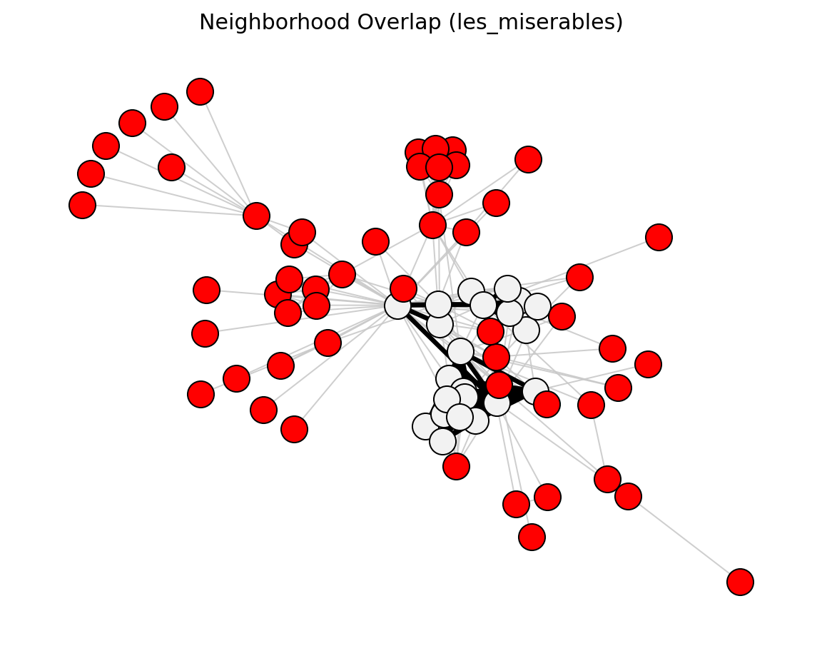
networkx_backbone.neighborhood_overlap(G)

Score each edge by the raw neighborhood overlap of its endpoints.

For each edge (u, v), the overlap is the number of common neighbors: |N(u) & N(v)|. The score is stored as the "overlap" edge attribute.

Parameters:

G (networkx.Graph or networkx.DiGraph) – Input graph. For directed graphs, neighborhoods are defined by successors (out-neighbors).

Returns:

H – Copy of G with the "overlap" edge attribute added.

Return type:

graph

Examples

>>> import networkx as nx
>>> from networkx_backbone import fraction_filter, neighborhood_overlap
>>> G = nx.les_miserables_graph()
>>> H = neighborhood_overlap(G)
>>> backbone = fraction_filter(H, "overlap", 0.3, ascending=False)
>>> backbone.number_of_edges() <= H.number_of_edges()
True

Computational complexity estimate is O(mn) time and O(n + m) space.

networkx_backbone.jaccard_backbone(G)

Score each edge by the Jaccard similarity of its endpoint neighborhoods.

For each edge (u, v):

\[J_{uv} = \frac{|N(u) \cap N(v)|}{|N(u) \cup N(v)|}\]

The score is stored as the "jaccard" edge attribute.

Parameters:

G (networkx.Graph or networkx.DiGraph) – Input graph.

Returns:

H – Copy of G with the "jaccard" edge attribute added.

Return type:

graph

References

[1]

Jaccard, P. (1901). Distribution de la flore alpine dans le bassin des Dranses et dans quelques regions voisines. Bulletin de la Societe Vaudoise des Sciences Naturelles, 37, 241-272.

Examples

>>> import networkx as nx
>>> from networkx_backbone import fraction_filter, jaccard_backbone
>>> G = nx.les_miserables_graph()
>>> H = jaccard_backbone(G)
>>> backbone = fraction_filter(H, "jaccard", 0.3, ascending=False)
>>> backbone.number_of_edges() <= H.number_of_edges()
True

Computational complexity estimate is O(mn) time and O(n + m) space.

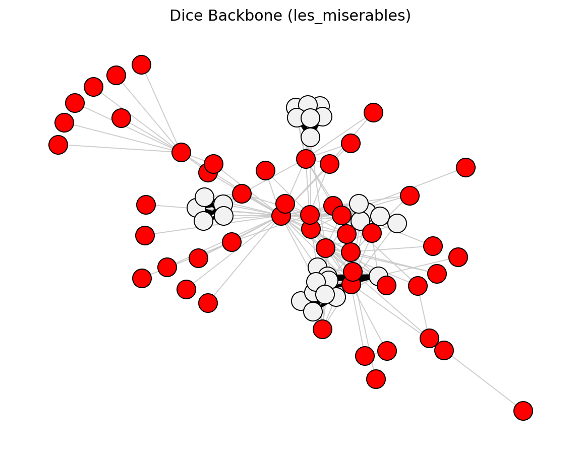
networkx_backbone.dice_backbone(G)

Score each edge by the Dice similarity of its endpoint neighborhoods.

For each edge (u, v):

\[D_{uv} = \frac{2 \, |N(u) \cap N(v)|}{k_u + k_v}\]

The score is stored as the "dice" edge attribute.

Parameters:

G (networkx.Graph or networkx.DiGraph) – Input graph.

Returns:

H – Copy of G with the "dice" edge attribute added.

Return type:

graph

References

[1]

Dice, L. R. (1945). Measures of the amount of ecologic association between species. Ecology, 26(3), 297-302.

Examples

>>> import networkx as nx
>>> from networkx_backbone import dice_backbone, fraction_filter
>>> G = nx.les_miserables_graph()
>>> H = dice_backbone(G)
>>> backbone = fraction_filter(H, "dice", 0.3, ascending=False)
>>> backbone.number_of_edges() <= H.number_of_edges()
True

Computational complexity estimate is O(mn) time and O(n + m) space.

networkx_backbone.cosine_backbone(G)

Score each edge by the cosine similarity of its endpoint neighborhoods.

For each edge (u, v):

\[C_{uv} = \frac{|N(u) \cap N(v)|}{\sqrt{k_u \, k_v}}\]

The score is stored as the "cosine" edge attribute.

Parameters:

G (networkx.Graph or networkx.DiGraph) – Input graph.

Returns:

H – Copy of G with the "cosine" edge attribute added.

Return type:

graph

References

[1]

Salton, G. & McGill, M. J. (1983). Introduction to Modern Information Retrieval. McGraw-Hill.

Examples

>>> import networkx as nx
>>> from networkx_backbone import cosine_backbone, fraction_filter
>>> G = nx.les_miserables_graph()
>>> H = cosine_backbone(G)
>>> backbone = fraction_filter(H, "cosine", 0.3, ascending=False)
>>> backbone.number_of_edges() <= H.number_of_edges()
True

Computational complexity estimate is O(mn) time and O(n + m) space.

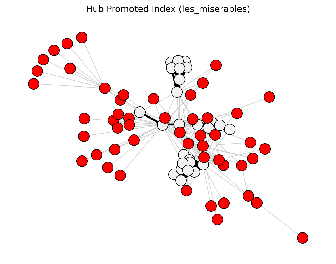
networkx_backbone.hub_promoted_index(G)

Score each edge by the Hub Promoted Index of its endpoint neighborhoods.

For each edge (u, v):

\[\mathrm{HPI}_{uv} = \frac{|N(u) \cap N(v)|}{\min(k_u,\, k_v)}\]

The score is stored as the "hpi" edge attribute.

Parameters:

G (networkx.Graph or networkx.DiGraph) – Input graph.

Returns:

H – Copy of G with the "hpi" edge attribute added.

Return type:

graph

References

[1]

Ravasz, E., Somera, A. L., Mongru, D. A., Oltvai, Z. N. & Barabasi, A.-L. (2002). Hierarchical organization of modularity in metabolic networks. Science, 297(5586), 1551-1555.

Examples

>>> import networkx as nx
>>> from networkx_backbone import fraction_filter, hub_promoted_index
>>> G = nx.les_miserables_graph()
>>> H = hub_promoted_index(G)
>>> backbone = fraction_filter(H, "hpi", 0.3, ascending=False)
>>> backbone.number_of_edges() <= H.number_of_edges()
True

Computational complexity estimate is O(mn) time and O(n + m) space.

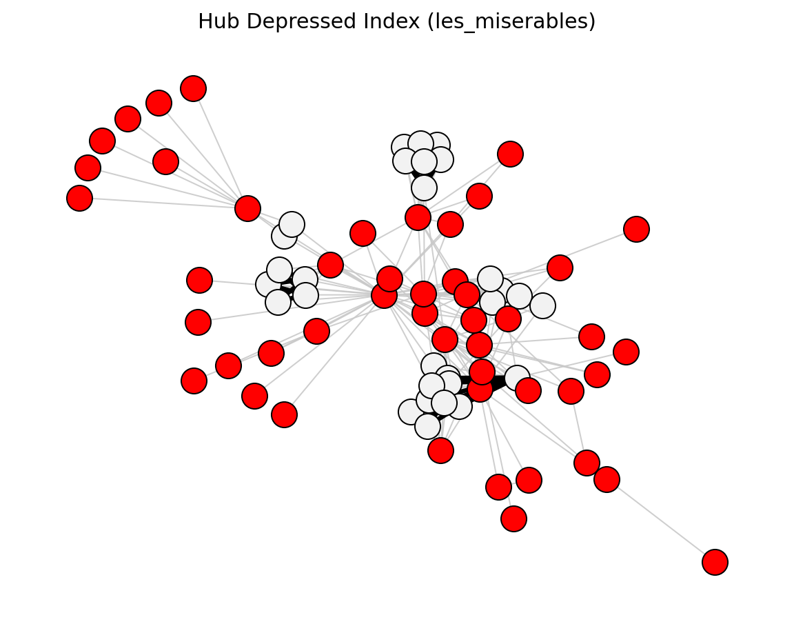
networkx_backbone.hub_depressed_index(G)

Score each edge by the Hub Depressed Index of its endpoint neighborhoods.

For each edge (u, v):

\[\mathrm{HDI}_{uv} = \frac{|N(u) \cap N(v)|}{\max(k_u,\, k_v)}\]

The score is stored as the "hdi" edge attribute.

Parameters:

G (networkx.Graph or networkx.DiGraph) – Input graph.

Returns:

H – Copy of G with the "hdi" edge attribute added.

Return type:

graph

References

[1]

Ravasz, E., Somera, A. L., Mongru, D. A., Oltvai, Z. N. & Barabasi, A.-L. (2002). Hierarchical organization of modularity in metabolic networks. Science, 297(5586), 1551-1555.

Examples

>>> import networkx as nx
>>> from networkx_backbone import fraction_filter, hub_depressed_index
>>> G = nx.les_miserables_graph()
>>> H = hub_depressed_index(G)
>>> backbone = fraction_filter(H, "hdi", 0.3, ascending=False)
>>> backbone.number_of_edges() <= H.number_of_edges()
True

Computational complexity estimate is O(mn) time and O(n + m) space.

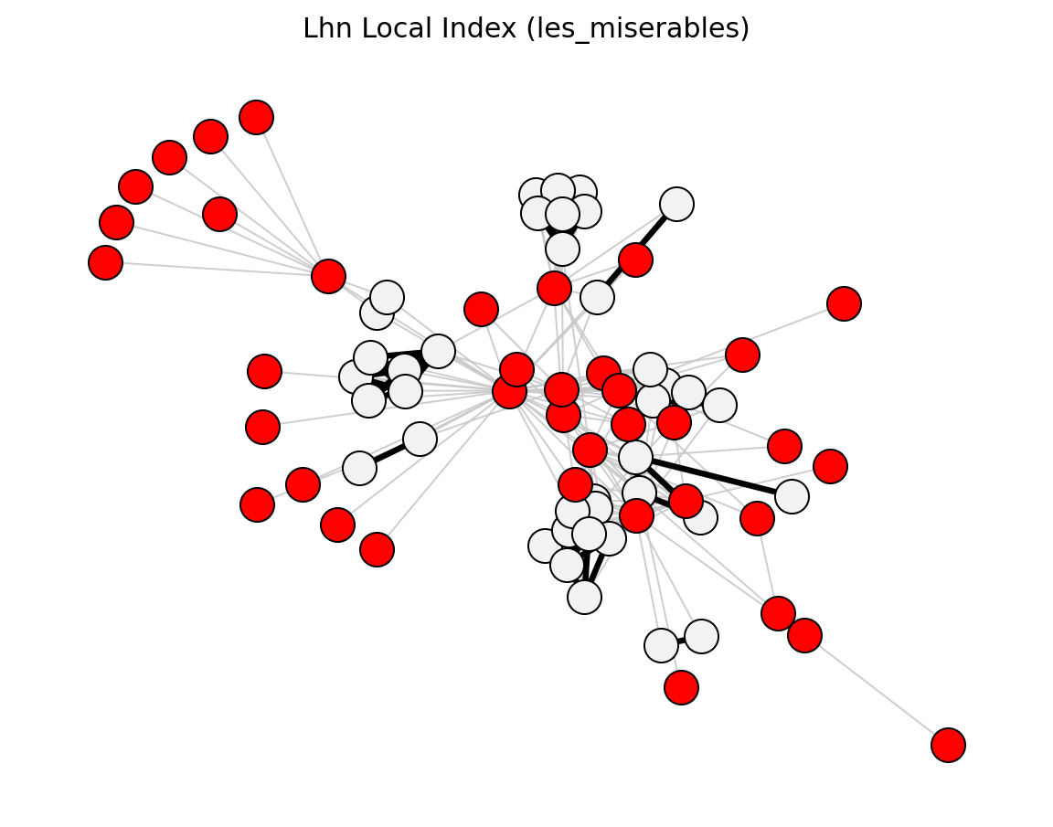
networkx_backbone.lhn_local_index(G)

Score each edge by the Leicht-Holme-Newman local similarity index.

For each edge (u, v):

\[\mathrm{LHN}_{uv} = \frac{|N(u) \cap N(v)|}{k_u \cdot k_v}\]

The score is stored as the "lhn_local" edge attribute.

Parameters:

G (networkx.Graph or networkx.DiGraph) – Input graph.

Returns:

H – Copy of G with the "lhn_local" edge attribute added.

Return type:

graph

References

[1]

Leicht, E. A., Holme, P. & Newman, M. E. J. (2006). Vertex similarity in networks. Physical Review E, 73(2), 026120.

Examples

>>> import networkx as nx
>>> from networkx_backbone import fraction_filter, lhn_local_index
>>> G = nx.les_miserables_graph()
>>> H = lhn_local_index(G)
>>> backbone = fraction_filter(H, "lhn_local", 0.3, ascending=False)
>>> backbone.number_of_edges() <= H.number_of_edges()
True

Computational complexity estimate is O(mn) time and O(n + m) space.

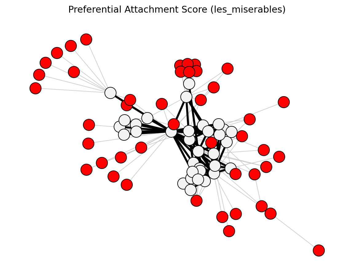
networkx_backbone.preferential_attachment_score(G)

Score each edge by the preferential attachment index.

For each edge (u, v):

\[\mathrm{PA}_{uv} = k_u \cdot k_v\]

The score is stored as the "pa" edge attribute.

Parameters:

G (networkx.Graph or networkx.DiGraph) – Input graph.

Returns:

H – Copy of G with the "pa" edge attribute added.

Return type:

graph

References

[1]

Barabasi, A.-L. & Albert, R. (1999). Emergence of scaling in random networks. Science, 286(5439), 509-512.

Examples

>>> import networkx as nx
>>> from networkx_backbone import fraction_filter, preferential_attachment_score
>>> G = nx.les_miserables_graph()
>>> H = preferential_attachment_score(G)
>>> backbone = fraction_filter(H, "pa", 0.3, ascending=False)
>>> backbone.number_of_edges() <= H.number_of_edges()
True

Computational complexity estimate is O(n + m) time and O(n + m) space.

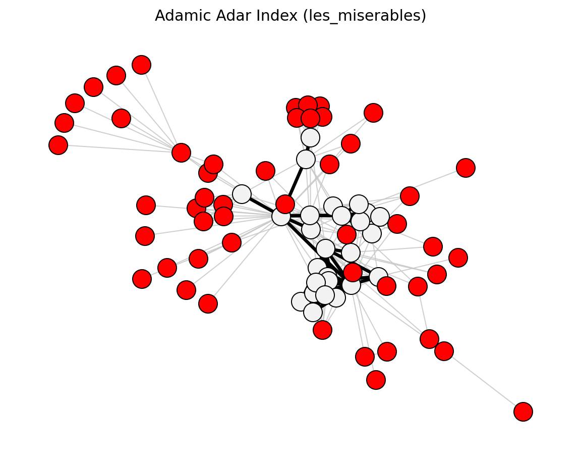
networkx_backbone.adamic_adar_index(G)

Score each edge by the Adamic-Adar index.

For each edge (u, v):

\[\mathrm{AA}_{uv} = \sum_{z \,\in\, N(u) \cap N(v)} \frac{1}{\log k_z}\]

The score is stored as the "adamic_adar" edge attribute.

Parameters:

G (networkx.Graph or networkx.DiGraph) – Input graph.

Returns:

H – Copy of G with the "adamic_adar" edge attribute added.

Return type:

graph

References

[1]

Adamic, L. A. & Adar, E. (2003). Friends and neighbors on the Web. Social Networks, 25(3), 211-230.

Examples

>>> import networkx as nx
>>> from networkx_backbone import adamic_adar_index, fraction_filter
>>> G = nx.les_miserables_graph()
>>> H = adamic_adar_index(G)
>>> backbone = fraction_filter(H, "adamic_adar", 0.3, ascending=False)
>>> backbone.number_of_edges() <= H.number_of_edges()
True

Computational complexity estimate is O(mn) time and O(n + m) space.

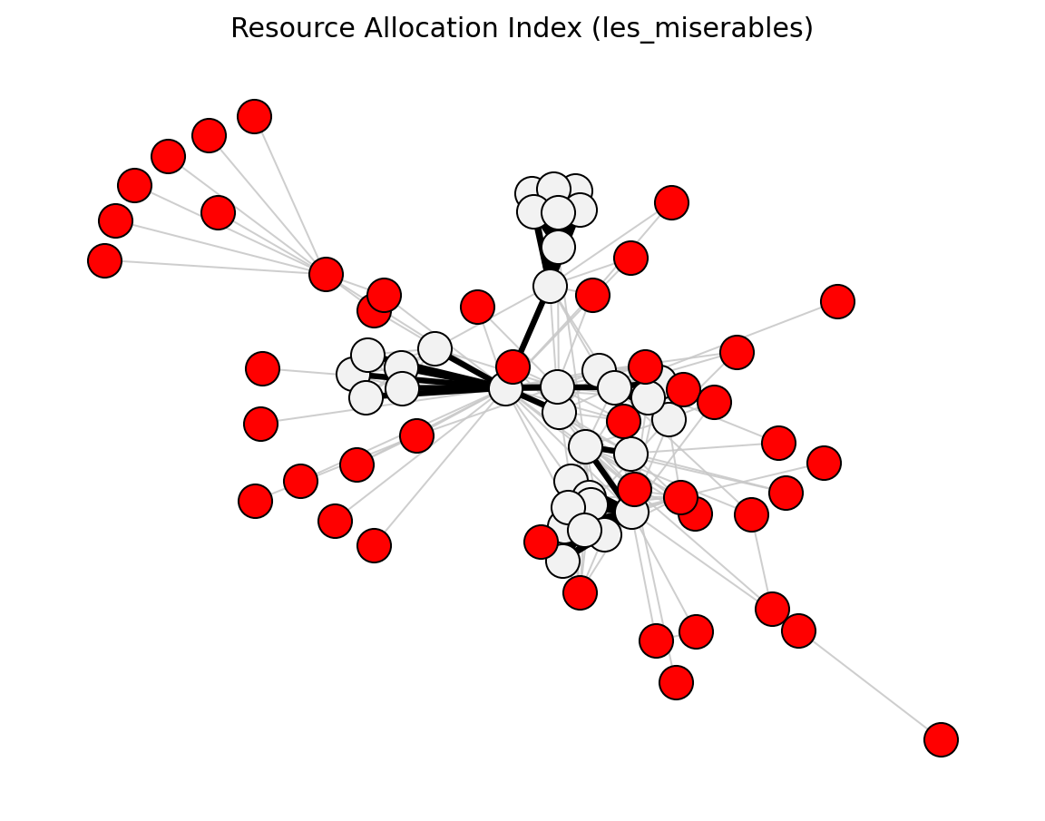
networkx_backbone.resource_allocation_index(G)

Score each edge by the resource-allocation index.

For each edge (u, v):

\[\mathrm{RA}_{uv} = \sum_{z \,\in\, N(u) \cap N(v)} \frac{1}{k_z}\]

The score is stored as the "resource_allocation" edge attribute.

Parameters:

G (networkx.Graph or networkx.DiGraph) – Input graph.

Returns:

H – Copy of G with the "resource_allocation" edge attribute added.

Return type:

graph

References

[1]

Zhou, T., Lu, L. & Zhang, Y.-C. (2009). Predicting missing links via local information. European Physical Journal B, 71(4), 623-630.

Examples

>>> import networkx as nx
>>> from networkx_backbone import fraction_filter, resource_allocation_index
>>> G = nx.les_miserables_graph()
>>> H = resource_allocation_index(G)
>>> backbone = fraction_filter(H, "resource_allocation", 0.3, ascending=False)
>>> backbone.number_of_edges() <= H.number_of_edges()
True

Computational complexity estimate is O(mn) time and O(n + m) space.

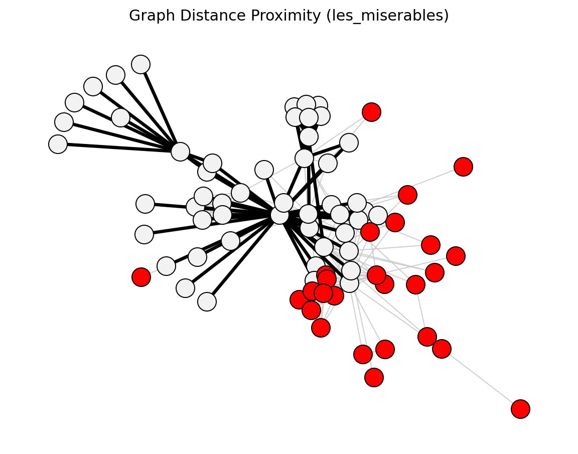
networkx_backbone.graph_distance_proximity(G, all_pairs=False)

Score edges by reciprocal shortest-path distance.

By default, scores are computed for existing edges only. With all_pairs=True, scores are computed for every node pair (all unordered pairs in undirected graphs; all ordered pairs in directed graphs, excluding self-pairs).

Parameters:

• G (networkx.Graph or networkx.DiGraph) – Input graph.

• all_pairs (bool, optional (default=False)) – If False, annotate only existing edges in a copy of G. If True, return a graph containing all node pairs as edges and annotate each with "dist".

Returns:

H – Graph with the "dist" edge attribute added.

Return type:

graph

References

[1]

Liben-Nowell, D. & Kleinberg, J. (2007). The link-prediction problem for social networks. JASIST, 58(7), 1019-1031.

Examples

>>> import networkx as nx
>>> from networkx_backbone import fraction_filter, graph_distance_proximity
>>> G = nx.les_miserables_graph()
>>> H = graph_distance_proximity(G)
>>> backbone = fraction_filter(H, "dist", 0.3, ascending=False)
>>> backbone.number_of_edges() <= H.number_of_edges()
True
>>> H_all = graph_distance_proximity(G, all_pairs=True)
>>> H_all.number_of_edges() >= H.number_of_edges()
True

Computational complexity estimate is O(n(n + m)) time and O(n^2 + m) space.

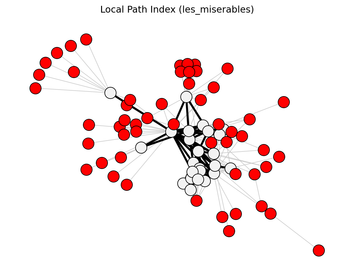
networkx_backbone.local_path_index(G, epsilon=0.01)

Score each edge by the local path index.

For each edge (u, v):

\[\mathrm{LP}_{uv} = (A^2)_{uv} + \varepsilon \, (A^3)_{uv}\]

where A is the adjacency matrix. The score is stored as the "lp" edge attribute.

Parameters:

• G (networkx.Graph or networkx.DiGraph) – Input graph.

• epsilon (float, optional (default=0.01)) – Weight for third-order paths.

Returns:

H – Copy of G with the "lp" edge attribute added.

Return type:

graph

References

[1]

Lu, L., Jin, C.-H. & Zhou, T. (2009). Similarity index based on local random walk and superposed with the AA index. EPL (Europhysics Letters), 89(1), 18001.

Examples

>>> import networkx as nx
>>> from networkx_backbone import fraction_filter, local_path_index
>>> G = nx.les_miserables_graph()
>>> H = local_path_index(G)
>>> backbone = fraction_filter(H, "lp", 0.3, ascending=False)
>>> backbone.number_of_edges() <= H.number_of_edges()
True

Computational complexity estimate is O(n^3) time and O(n^2) space.

Gallery Examples

Score-Then-Filter Graph Comparison Gallery

Score-Then-Filter Graph Comparison Gallery

Function Image Reference

neighborhood_overlap()

jaccard_backbone()

dice_backbone()

cosine_backbone()

hub_promoted_index()

hub_depressed_index()

lhn_local_index()

preferential_attachment_score()

adamic_adar_index()

resource_allocation_index()

graph_distance_proximity()

local_path_index()