Bipartite Methods#
Examples in this module use nx.davis_southern_women_graph().
Projection scoring methods return full graphs with p-values/weights; use
threshold_filter() or
boolean_filter() as needed.
Complexity classes are provided in each function docstring.
Bipartite projection backbone methods.
These methods operate on bipartite networks and extract significant edges in the one-mode projection among “agent” nodes.
- networkx_backbone.simple_projection(B, agent_nodes, weight='weight')[source]#
Project a bipartite graph using shared-neighbor counts.
For agent nodes
uandv, the weight is|Gamma(u) ∩ Gamma(v)|.References
[1]Coscia, M. & Neffke, F. (2017). Network backboning with noisy data. arXiv:1906.09081.
Computational complexity estimate is
O(n_a^2 n_f + e_b)time andO(n_a n_f + n_a^2)space.
- networkx_backbone.hyper_projection(B, agent_nodes, weight='weight')[source]#
Project a bipartite graph using hyperbolic weighting.
For agent nodes
uandv, the weight issum_{z in Gamma(u) ∩ Gamma(v)} 1 / d(z)whered(z)is the artifact degree.References
[1]Coscia, M. & Neffke, F. (2017). Network backboning with noisy data. arXiv:1906.09081.
Computational complexity estimate is
O(n_a^2 n_f + e_b)time andO(n_a n_f + n_a^2)space.
- networkx_backbone.probs_projection(B, agent_nodes, weight='weight', directed=False)[source]#
Project a bipartite graph using ProbS random-walk weights.
The directed score from
utovis(1 / d(u)) * sum_{z in Gamma(u) ∩ Gamma(v)} 1 / d(z).References
[1]Coscia, M. & Neffke, F. (2017). Network backboning with noisy data. arXiv:1906.09081.
Computational complexity estimate is
O(n_a^2 n_f + e_b)time andO(n_a n_f + n_a^2)space.
- networkx_backbone.ycn_projection(B, agent_nodes, weight='weight', directed=False, max_iter=1000, tol=1e-12)[source]#
Project a bipartite graph using YCN random-walk stationary flow.
This method estimates a random-walk transition matrix on the projected layer and scores pairs by stationary flow
pi_u * T_uv.References
[1]Coscia, M. & Neffke, F. (2017). Network backboning with noisy data. arXiv:1906.09081.
Computational complexity estimate is
O(n_a^2 n_f + I n_a^2 + e_b)time andO(n_a n_f + n_a^2)space.
- networkx_backbone.bipartite_projection(B, agent_nodes, method='simple', weight='weight', directed=False, max_iter=1000, tol=1e-12)[source]#
Dispatch weighted bipartite projections by method name.
Supported methods are
"simple","hyper","probs", and"ycn".Computational complexity estimate is
O(n_a^2 n_f + I n_a^2 + e_b)time andO(n_a n_f + n_a^2)space.
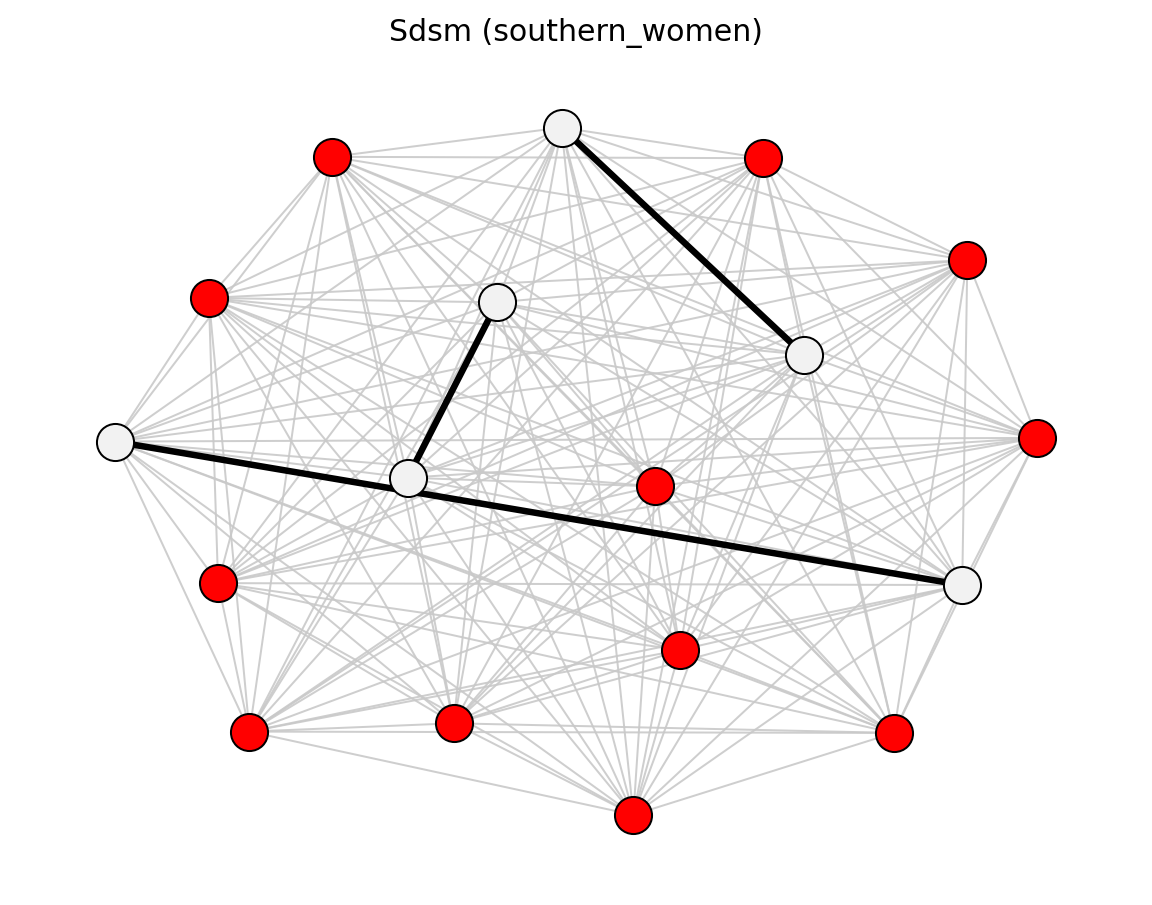
- networkx_backbone.sdsm(B, agent_nodes, alpha=0.05, weight=None, projection='simple', projection_weight='weight', projection_directed=False, projection_max_iter=1000, projection_tol=1e-12)[source]#
Extract a backbone from a bipartite projection using the SDSM.
The Stochastic Degree Sequence Model [1] generates random bipartite networks that preserve the row and column sums on average (as probabilities). The p-value for each pair of agents is computed analytically using a Poisson-binomial approximation (normal).
- Parameters:
B (graph) – A bipartite NetworkX graph.
agent_nodes (iterable) – Nodes in the “agent” partition.
alpha (float, optional (default=0.05)) – Retained for API compatibility. This function returns the full projected graph with p-values on all edges; apply
threshold_filter()to select significant edges.weight (None or string, optional (default=None)) – Not used for SDSM (bipartite is unweighted); reserved for API consistency.
projection ({"simple", "hyper", "probs", "ycn"}, optional) – Projection weighting assigned to each returned edge.
projection_weight (str, optional) – Edge attribute name for the projection weight.
projection_directed (bool, optional) – Whether to use directed projection scores. Not supported for the undirected backbone output.
projection_max_iter (int, optional) – Maximum iterations for
projection="ycn".projection_tol (float, optional) – Convergence tolerance for
projection="ycn".
- Returns:
backbone – Full unipartite projection among agent nodes. Each edge has a
"sdsm_pvalue"attribute and projection weights.- Return type:
graph
- Raises:
NetworkXError – If B is not bipartite or agent_nodes contains nodes not in B.
References
[1]Neal, Z. P. (2014). The backbone of bipartite projections: Inferring relationships from co-authorship, co-sponsorship, co-attendance and other co-behaviors. Social Networks, 39, 84-97.
Examples
>>> import networkx as nx
>>> from networkx_backbone import sdsm
>>> B = nx.davis_southern_women_graph()
>>> women = [n for n, d in B.nodes(data=True) if d["bipartite"] == 0]
>>> scored = sdsm(B, agent_nodes=women)
>>> from networkx_backbone import threshold_filter
>>> backbone = threshold_filter(scored, "sdsm_pvalue", 0.05, mode="below")
>>> all("sdsm_pvalue" in data for _, _, data in backbone.edges(data=True))
True
Computational complexity estimate is
O(n_a^2 n_f + e_b)time andO(n_a n_f + n_a^2)space.
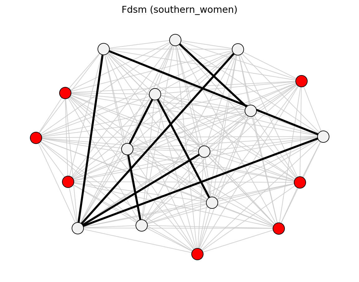
- networkx_backbone.fdsm(B, agent_nodes, alpha=0.05, trials=1000, seed=None, projection='simple', projection_weight='weight', projection_directed=False, projection_max_iter=1000, projection_tol=1e-12)[source]#
Extract a backbone from a bipartite projection using the FDSM.
The Fixed Degree Sequence Model [1] uses Monte Carlo simulation to estimate p-values. Each trial generates a random bipartite graph that exactly preserves both the row sums (agent degrees) and column sums (artifact degrees), then computes the co-occurrence matrix.
- Parameters:
B (graph) – A bipartite NetworkX graph.
agent_nodes (iterable) – Nodes in the “agent” partition.
alpha (float, optional (default=0.05)) – Retained for API compatibility. This function returns the full projected graph with p-values on all edges; apply
threshold_filter()to select significant edges.trials (int, optional (default=1000)) – Number of Monte Carlo randomisations.
seed (integer, random_state, or None (default)) – Random seed for reproducibility.
projection ({"simple", "hyper", "probs", "ycn"}, optional) – Projection weighting assigned to each returned edge.
projection_weight (str, optional) – Edge attribute name for the projection weight.
projection_directed (bool, optional) – Whether to use directed projection scores. Not supported for the undirected backbone output.
projection_max_iter (int, optional) – Maximum iterations for
projection="ycn".projection_tol (float, optional) – Convergence tolerance for
projection="ycn".
- Returns:
backbone – Full unipartite projection among agent nodes. Each edge has an
"fdsm_pvalue"attribute and projection weights.- Return type:
graph
- Raises:
NetworkXError – If B is not bipartite or agent_nodes contains nodes not in B.
References
[1]Neal, Z. P., Domagalski, R., & Sagan, B. (2021). Comparing alternatives to the fixed degree sequence model. Scientific Reports, 11, 23929.
Examples
>>> import networkx as nx
>>> from networkx_backbone import fdsm
>>> B = nx.davis_southern_women_graph()
>>> women = [n for n, d in B.nodes(data=True) if d["bipartite"] == 0]
>>> scored = fdsm(B, agent_nodes=women, trials=100, seed=42)
>>> from networkx_backbone import threshold_filter
>>> backbone = threshold_filter(scored, "fdsm_pvalue", 0.05, mode="below")
>>> all("fdsm_pvalue" in data for _, _, data in backbone.edges(data=True))
True
Computational complexity estimate is
O(T n_a^2 n_f + e_b)time andO(n_a n_f + n_a^2)space.
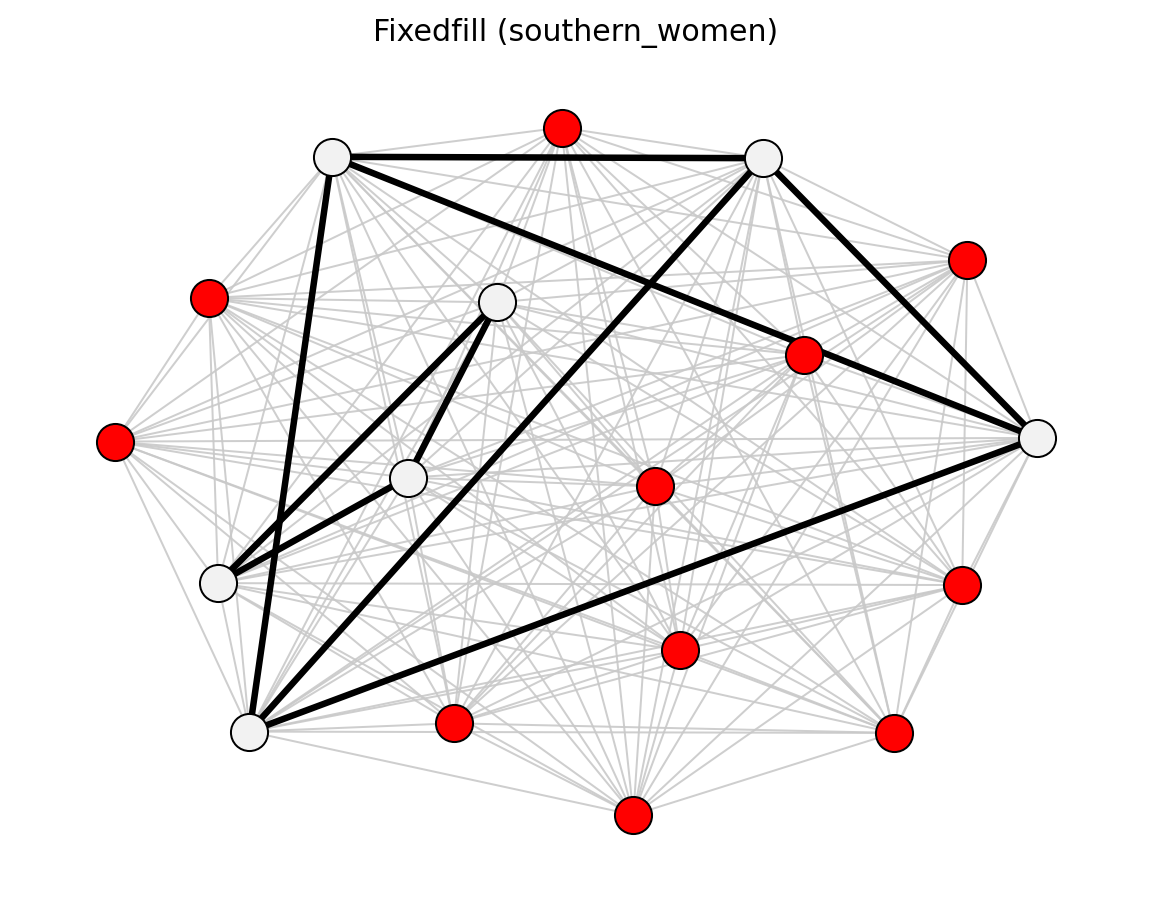
- networkx_backbone.fixedfill(B, agent_nodes, alpha=0.05, projection='simple', projection_weight='weight', projection_directed=False, projection_max_iter=1000, projection_tol=1e-12)[source]#
Backbone from a fixed-fill null model for bipartite projections.
Under the null, each bipartite cell is occupied independently with probability equal to the observed fill rate.
Computational complexity estimate is
O(n_a^2 n_f + e_b)time andO(n_a n_f + n_a^2)space.
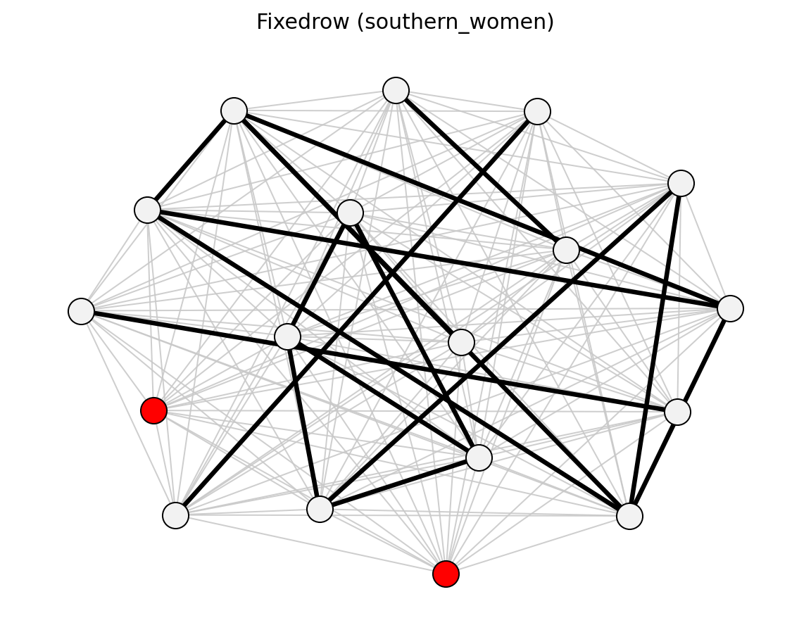
- networkx_backbone.fixedrow(B, agent_nodes, alpha=0.05, projection='simple', projection_weight='weight', projection_directed=False, projection_max_iter=1000, projection_tol=1e-12)[source]#
Backbone from a fixed-row null model for bipartite projections.
Computational complexity estimate is
O(n_a^2 n_f + e_b)time andO(n_a n_f + n_a^2)space.
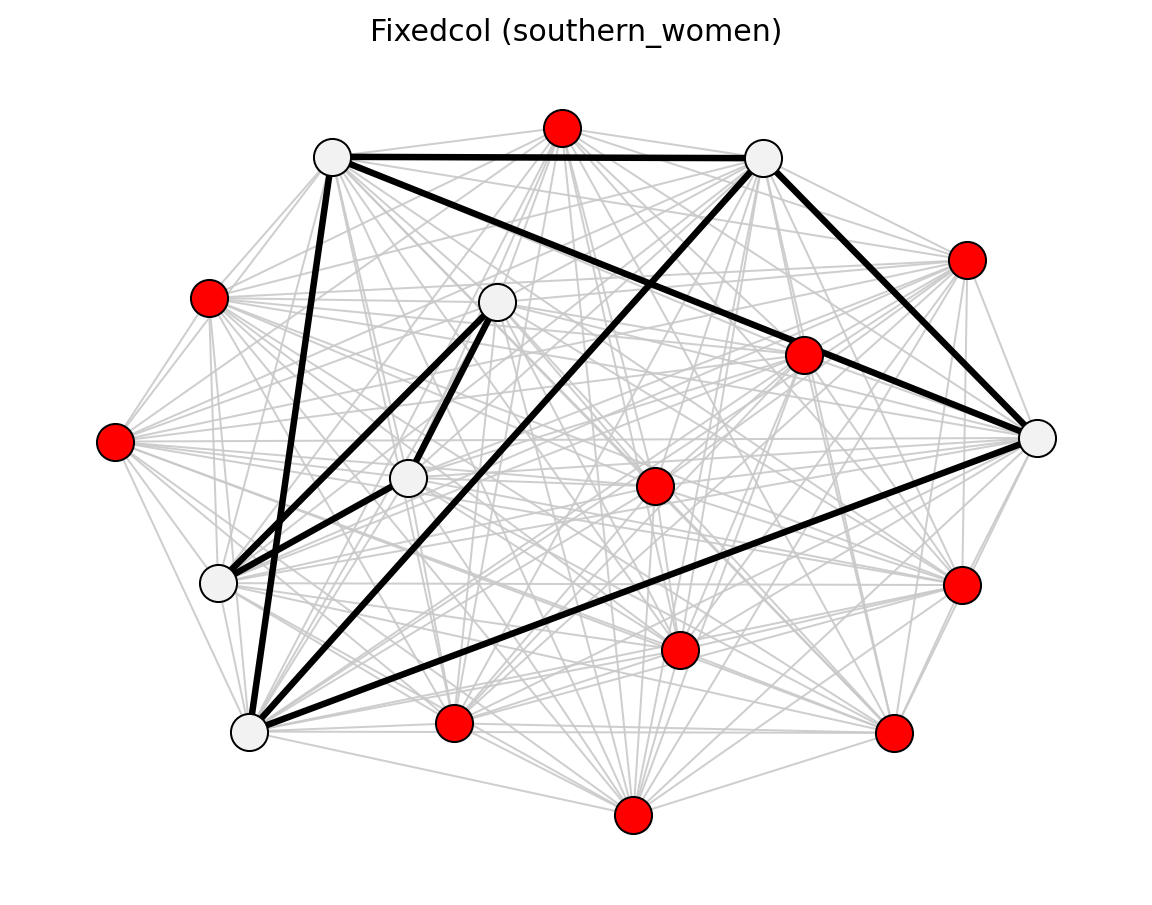
- networkx_backbone.fixedcol(B, agent_nodes, alpha=0.05, projection='simple', projection_weight='weight', projection_directed=False, projection_max_iter=1000, projection_tol=1e-12)[source]#
Backbone from a fixed-column null model for bipartite projections.
Computational complexity estimate is
O(n_a^2 n_f + e_b)time andO(n_a n_f + n_a^2)space.
- networkx_backbone.bicm(B, agent_nodes, return_labels=False)[source]#
Estimate Bipartite Configuration Model edge probabilities.
- Parameters:
B (graph) – A bipartite NetworkX graph.
agent_nodes (iterable) – Nodes in the “agent” partition.
return_labels (bool, optional (default=False)) – If
True, also return(agents, artifacts)labels.
- Returns:
P (np.ndarray) – Probability matrix of shape
(n_agents, n_artifacts)whereP[i, k]is the estimated probability of an edge between agentiand artifactk.(P, agents, artifacts) (tuple) – Returned when
return_labels=True.Computational complexity estimate is
O(n_a n_f + e_b)time andO(n_a n_f)space.
- networkx_backbone.fastball(matrix, n_swaps=None, seed=None)[source]#
Randomize a binary matrix while preserving row and column sums.
This is a Curveball-style randomizer commonly used for bipartite null-model generation.
- Parameters:
matrix (array-like) – Binary matrix with shape
(n_rows, n_cols).n_swaps (int or None, optional) – Number of row-pair trades. Defaults to
5 * n_rows.seed (integer, random_state, or None) – Random seed for reproducibility.
- Returns:
randomized (np.ndarray) – Randomized binary matrix with preserved row/column sums.
Computational complexity estimate is
O(r c + S c)time andO(r c)space.
Gallery Examples#
Function Image Reference
High-Level Wrappers
- networkx_backbone.backbone_from_projection(B, agent_nodes=None, method='sdsm', alpha=0.05, projection='simple', projection_weight='weight', projection_directed=False, projection_max_iter=1000, projection_tol=1e-12, **kwargs)[source]#
Extract a projection backbone using a method-name dispatch wrapper.
- Parameters:
projection ({"simple", "hyper", "probs", "ycn"}, optional) – Bipartite projection weighting to assign to returned edges.
projection_weight (str, optional) – Edge attribute name used for projection weights.
projection_directed (bool, optional) – Whether to use directed projection weights. Undirected backbones do not support directed projections and will raise an error if
True.projection_max_iter (int, optional) – Maximum iterations for
projection="ycn"stationary distribution estimation.projection_tol (float, optional) – Convergence tolerance for
projection="ycn".space. (Computational complexity estimate is O(T n_a^2 n_f + e_b) time and O(n_a n_f + n_a^2))
- networkx_backbone.backbone_from_weighted(G, method='disparity', weight='weight', alpha=0.05, collapse_multiedges=True, edge_type_attr=None, **kwargs)[source]#
Extract a weighted-network backbone using method-name dispatch.
Multi-edge inputs can be collapsed automatically before scoring.
- Parameters:
collapse_multiedges (bool, optional (default=True)) – If
TrueandGis aMultiGraphorMultiDiGraph, collapse parallel edges usingmultigraph_to_weighted().edge_type_attr (string or None, optional (default=None)) – Edge attribute used when collapsing multi-edges. If provided, edge weights count distinct edge types per node pair; otherwise they count parallel edges.
space. (Computational complexity estimate is O(m log n) time and O(n + m))